 Products Home / Optical Systems / Objective Lenses, Scan Lenses, and Tube Lenses / High-Power MicroSpot® Focusing Objectives for UV Lasers
High-Power MicroSpot® Focusing Objectives for UV Lasers
- Excimer-Grade UV Fused Silica and CaF2 Lens Elements
- Air-Spaced Designs with High Damage Thresholds
- AR Coatings to Optimize Transmission
- 3X to 50X Magnifications Available
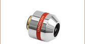
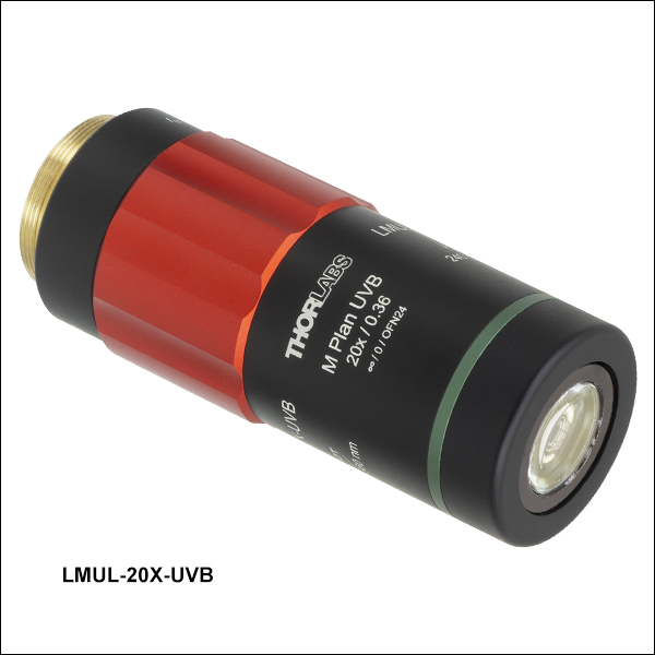
LMUL-20X-UVB
20X, Long Working Distance, UV Achromatic Objective
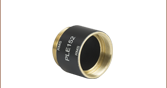
LMU-40X-NUV
40X, UV Achromatic Objective
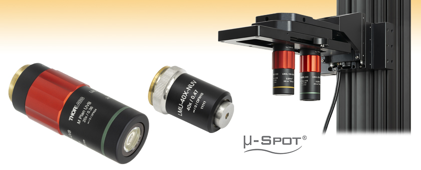
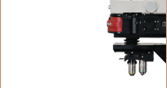
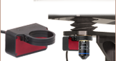
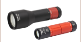
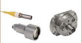
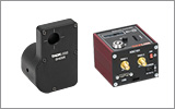
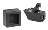
Application Idea
Two Focusing Objectives Mounted in a CSN200 Dual-Objective Nosepiece
Through Use of a Thread Adapter


Please Wait
| Objective Lens Selection Guide |
|---|
| Objectives |
| Super Apochromatic Microscope Objectives Microscopy Objectives, Dry Microscopy Objectives, Oil Immersion Physiology Objectives, Water Dipping or Immersion Phase Contrast Objectives Long Working Distance Objectives Reflective Microscopy Objectives UV Focusing Objectives VIS and NIR Focusing Objectives |
| Scan Lenses and Tube Lenses |
| Scan Lenses F-Theta Scan Lenses Infinity-Corrected Tube Lenses |
 Zemax Files Zemax Files |
|---|
| Click on the red Document icon next to the item numbers below to access the Zemax file download. Our entire Zemax Catalog is also available. |
Click to Enlarge
This diagram illustrates the labels, working distance, and parfocal distance. The format of the engraved specifications will vary between objectives and manufacturers. (See the Objective Tutorial tab for more information about microscope objective types.)
Features
- Theoretical Focus Spot Size: ≤5 µm
- Entrance Aperture: ≥3.4 mm
- Infinite Conjugate Design
- Threaded Housings
- Air-Spaced Design
Applications
- Laser Engraving
- Laser Cutting
- 3D Photolithography
- 3D Printing
- Wafer Dicing and Inspection
- Laser Induced Breakdown Spectroscopy (LIBS)
Thorlabs' High-Power UV MicroSpot® Focusing Objectives are designed for use with UV excimer lasers and other ultraviolet sources in on-axis laser focusing and microimaging applications. The objectives contain lens elements made from high-quality, low-absorption, excimer-grade fused silica and CaF2. These lenses are AR coated and optically designed for narrowband or broadband wavelength ranges (see the focal shift and AR coating performance graphs below). The objectives feature W26 x 0.706 or RMS (0.800"-36) threading; to use these objectives with a different thread standard, please see our microscope objective thread adapters.
Focusing objectives can be used in a variety of applications where intense optical power is necessary. Focused excimer sources in particular have uses in eye surgery, photolithography, and industrial laser cutting. Each section below lists some ideal applications for each group of our objectives. When incorporating these objectives into a system, note that the specified magnification for each objective is calculated assuming use with a 200 mm focal length tube lens, such as the TTL200-UVB.
The graphs below show the transmission and focal length shifts (FLS) for our MicroSpot® UV Focusing Objectives. Transmission graphs show the total transmission through each objective. The shaded regions indicate the wavelength range for the AR coating applied to the elements of each objective.
Long Working Distance, Achromatic UV Focusing Objective
Click to Enlarge
Click Here for Raw Data
The shaded region of this graph identifies the specified wavelength range of the AR coating.
Thorlabs offers custom V-coatings for our LMUL objectives upon request. These coatings can be designed to provide peak performance at select laser wavelengths while still giving moderate transmission at visible wavelengths. The axial focal length shift given above will still be valid for the given magnification of the custom objective. Contact Tech Support to request quotes and lead times for these custom coatings.
| Custom AR Coating Options for Long Working Distance Objectives | ||||
|---|---|---|---|---|
| Coating Type | Broadband NUV | 248 nm Center Wavelength | 266 nm Center Wavelength | 355 nm Center Wavelength |
| Reflectance Per Surface | <1.0% (325 nm - 500 nm) | <0.5% (240 nm - 260 nm) | <0.7% (248 nm - 287 nm) <0.2% (256 nm - 275 nm) |
<0.7% (325 nm - 380 nm) <0.2% (335 nm - 362 nm) |
| Total Transmission (Theoretical) |
||||
Achromatic UV Focusing Objectives
Click to Enlarge
Click Here for Raw Data
The shaded region of this graph identifies the specified wavelength range of the AR coating.
Click to Enlarge
Click Here for Raw Data
The shaded region of this graph identifies the specified wavelength range of the AR coating.
Narrowband UV Focusing Objectives
Click to Enlarge
Click Here for Raw Data
The shaded region of this graph identifies the specified wavelength range of the AR coating.
Click to Enlarge
Click Here for Raw Data
The shaded region of this graph identifies the specified wavelength range of the AR coating.

Narrowband UV Focusing Objectives with Laser Line AR Coatings
Click to Enlarge
Click Here for Raw Data
The shaded region of this graph identifies the specified wavelength range of the AR coating.
Click to Enlarge
Click Here for Raw Data
The shaded region of this graph identifies the specified wavelength range of the AR coating.
Click to Enlarge
Click Here for Raw Data
The shaded region of this graph identifies the specified wavelength range of the AR coating.
Click to Enlarge
Click Here for Raw Data
The shaded region of this graph identifies the specified wavelength range of the AR coating.
| Chromatic Aberration Correction per ISO Standard 19012-2 | ||
|---|---|---|
| Objective Class | Common Abbreviations | Axial Focal Shift Tolerancesa |
| Achromat | ACH, ACHRO, ACHROMAT | |δC' - δF'| ≤ 2 x δob |
| Semiapochromat (or Fluorite) |
SEMIAPO, FL, FLU | |δC' - δF'| ≤ 2 x δob |δF' - δe| ≤ 2.5 x δob |δC' - δe| ≤ 2.5 x δob |
| Apochromat | APO | |δC' - δF'| ≤ 2 x δob |δF' - δe| ≤ δob |δC' - δe| ≤ δob |
| Super Apochromat | SAPO | See Footnote b |
| Improved Visible Apochromat | VIS+ | See Footnotes b and c |
Parts of a Microscope Objective
Click on each label for more details.
This microscope objective serves only as an example. The features noted above with an asterisk may not be present on all objectives; they may be added, relocated, or removed from objectives based on the part's needs and intended application space.
Objective Tutorial
This tutorial describes features and markings of objectives and what they tell users about an objective's performance.
Objective Class and Aberration Correction
Objectives are commonly divided by their class. An objective's class creates a shorthand for users to know how the objective is corrected for imaging aberrations. There are two types of aberration corrections that are specified by objective class: field curvature and chromatic aberration.
Field curvature (or Petzval curvature) describes the case where an objective's plane of focus is a curved spherical surface. This aberration makes widefield imaging or laser scanning difficult, as the corners of an image will fall out of focus when focusing on the center. If an objective's class begins with "Plan", it will be corrected to have a flat plane of focus.
Images can also exhibit chromatic aberrations, where colors originating from one point are not focused to a single point. To strike a balance between an objective's performance and the complexity of its design, some objectives are corrected for these aberrations at a finite number of target wavelengths.
Five objective classes are shown in the table to the right; only three common objective classes are defined under the International Organization for Standards ISO 19012-2: Microscopes -- Designation of Microscope Objectives -- Chromatic Correction. Due to the need for better performance, we have added two additional classes that are not defined in the ISO classes.
Immersion Methods
Click on each image for more details.
Objectives can be divided by what medium they are designed to image through. Dry objectives are used in air; whereas dipping and immersion objectives are designed to operate with a fluid between the objective and the front element of the sample.
| Glossary of Terms | |
|---|---|
| Back Focal Length and Infinity Correction | The back focal length defines the location of the intermediate image plane. Most modern objectives will have this plane at infinity, known as infinity correction, and will signify this with an infinity symbol (∞). Infinity-corrected objectives are designed to be used with a tube lens between the objective and eyepiece. Along with increasing intercompatibility between microscope systems, having this infinity-corrected space between the objective and tube lens allows for additional modules (like beamsplitters, filters, or parfocal length extenders) to be placed in the beam path. Note that older objectives and some specialty objectives may have been designed with finite back focal lengths. In their inception, finite back focal length objectives were meant to interface directly with the objective's eyepiece. |
| Entrance Pupil Diameter (EP) | The entrance pupil diameter (EP), sometimes referred to as the entrance aperture diameter, corresponds to the appropriate beam diameter one should use to allow the objective to function properly. EP = 2 × NA × Effective Focal Length |
| Field Number (FN) and Field of View (FOV) |
The field number corresponds to the diameter of the field of view in object space (in millimeters) multiplied by the objective's magnification. Field Number = Field of View Diameter × Magnification |
| Magnification (M) | The magnification (M) of an objective is the lens tube focal length (L) divided by the objective's effective focal length (F). Effective focal length is sometimes abbreviated EFL: M = L / EFL . The total magnification of the system is the magnification of the objective multiplied by the magnification of the eyepiece or camera tube. The specified magnification on the microscope objective housing is accurate as long as the objective is used with a compatible tube lens focal length. Objectives will have a colored ring around their body to signify their magnification. This is fairly consistent across manufacturers; see the Parts of a Microscope Objective section for more details. |
| Numerical Aperture (NA) | Numerical aperture, a measure of the acceptance angle of an objective, is a dimensionless quantity. It is commonly expressed as: NA = ni × sinθa where θa is the maximum 1/2 acceptance angle of the objective, and ni is the index of refraction of the immersion medium. This medium is typically air, but may also be water, oil, or other substances. |
| Working Distance (WD) |
The working distance, often abbreviated WD, is the distance between the front element of the objective and the top of the specimen (in the case of objectives that are intended to be used without a cover glass) or top of the cover glass, depending on the design of the objective. The cover glass thickness specification engraved on the objective designates whether a cover glass should be used. |
A cover glass, or coverslip, is a small, thin sheet of glass that can be placed on a wet sample to create a flat surface to image across.
The most common, a standard #1.5 cover glass, is designed to be 0.17 mm thick. Due to variance in the manufacturing process the actual thickness may be different. The correction collar present on select objectives is used to compensate for cover glasses of different thickness by adjusting the relative position of internal optical elements. Note that many objectives do not have a variable cover glass correction, in which case the objectives have no correction collar. For example, an objective could be designed for use with only a #1.5 cover glass. This collar may also be located near the bottom of the objective, instead of the top as shown in the diagram.
Click to Enlarge
The graph above shows the magnitude of spherical aberration versus the thickness of the coverslip used for 632.8 nm light. For the typical coverslip thickness of 0.17 mm, the spherical aberration caused by the coverslip does not exceed the diffraction-limited aberration for objectives with NA up to 0.40.
When viewing an image with a camera, the system magnification is the product of the objective and camera tube magnifications. When viewing an image with trinoculars, the system magnification is the product of the objective and eyepiece magnifications.

| Manufacturer | Tube Lens Focal Length |
|---|---|
| Leica | f = 200 mm |
| Mitutoyo | f = 200 mm |
| Nikon | f = 200 mm |
| Olympus | f = 180 mm |
| Thorlabs | f = 200 mm |
| Zeiss | f = 165 mm |
Magnification and Sample Area Calculations
Magnification
The magnification of a system is the multiplicative product of the magnification of each optical element in the system. Optical elements that produce magnification include objectives, camera tubes, and trinocular eyepieces, as shown in the drawing to the right. It is important to note that the magnification quoted in these products' specifications is usually only valid when all optical elements are made by the same manufacturer. If this is not the case, then the magnification of the system can still be calculated, but an effective objective magnification should be calculated first, as described below.
To adapt the examples shown here to your own microscope, please use our Magnification and FOV Calculator, which is available for download by clicking on the red button above. Note the calculator is an Excel spreadsheet that uses macros. In order to use the calculator, macros must be enabled. To enable macros, click the "Enable Content" button in the yellow message bar upon opening the file.
Example 1: Camera Magnification
When imaging a sample with a camera, the image is magnified by the objective and the camera tube. If using a 20X Nikon objective and a 0.75X Nikon camera tube, then the image at the camera has 20X × 0.75X = 15X magnification.
Example 2: Trinocular Magnification
When imaging a sample through trinoculars, the image is magnified by the objective and the eyepieces in the trinoculars. If using a 20X Nikon objective and Nikon trinoculars with 10X eyepieces, then the image at the eyepieces has 20X × 10X = 200X magnification. Note that the image at the eyepieces does not pass through the camera tube, as shown by the drawing to the right.
Using an Objective with a Microscope from a Different Manufacturer
Magnification is not a fundamental value: it is a derived value, calculated by assuming a specific tube lens focal length. Each microscope manufacturer has adopted a different focal length for their tube lens, as shown by the table to the right. Hence, when combining optical elements from different manufacturers, it is necessary to calculate an effective magnification for the objective, which is then used to calculate the magnification of the system.
The effective magnification of an objective is given by Equation 1:
 |
(Eq. 1) |
Here, the Design Magnification is the magnification printed on the objective, fTube Lens in Microscope is the focal length of the tube lens in the microscope you are using, and fDesign Tube Lens of Objective is the tube lens focal length that the objective manufacturer used to calculate the Design Magnification. These focal lengths are given by the table to the right.
Note that Leica, Mitutoyo, Nikon, and Thorlabs use the same tube lens focal length; if combining elements from any of these manufacturers, no conversion is needed. Once the effective objective magnification is calculated, the magnification of the system can be calculated as before.
Example 3: Trinocular Magnification (Different Manufacturers)
When imaging a sample through trinoculars, the image is magnified by the objective and the eyepieces in the trinoculars. This example will use a 20X Olympus objective and Nikon trinoculars with 10X eyepieces.
Following Equation 1 and the table to the right, we calculate the effective magnification of an Olympus objective in a Nikon microscope:
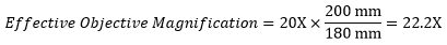 |
The effective magnification of the Olympus objective is 22.2X and the trinoculars have 10X eyepieces, so the image at the eyepieces has 22.2X × 10X = 222X magnification.
Sample Area When Imaged on a Camera
When imaging a sample with a camera, the dimensions of the sample area are determined by the dimensions of the camera sensor and the system magnification, as shown by Equation 2.
 |
(Eq. 2) |
The camera sensor dimensions can be obtained from the manufacturer, while the system magnification is the multiplicative product of the objective magnification and the camera tube magnification (see Example 1). If needed, the objective magnification can be adjusted as shown in Example 3.
As the magnification increases, the resolution improves, but the field of view also decreases. The dependence of the field of view on magnification is shown in the schematic to the right.
Example 4: Sample Area
The dimensions of the camera sensor in Thorlabs' previous-generation 1501M-USB Scientific Camera are 8.98 mm × 6.71 mm. If this camera is used with the Nikon objective and trinoculars from Example 1, which have a system magnification of 15X, then the image area is:
 |
Sample Area Examples
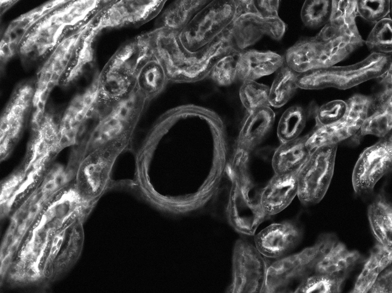
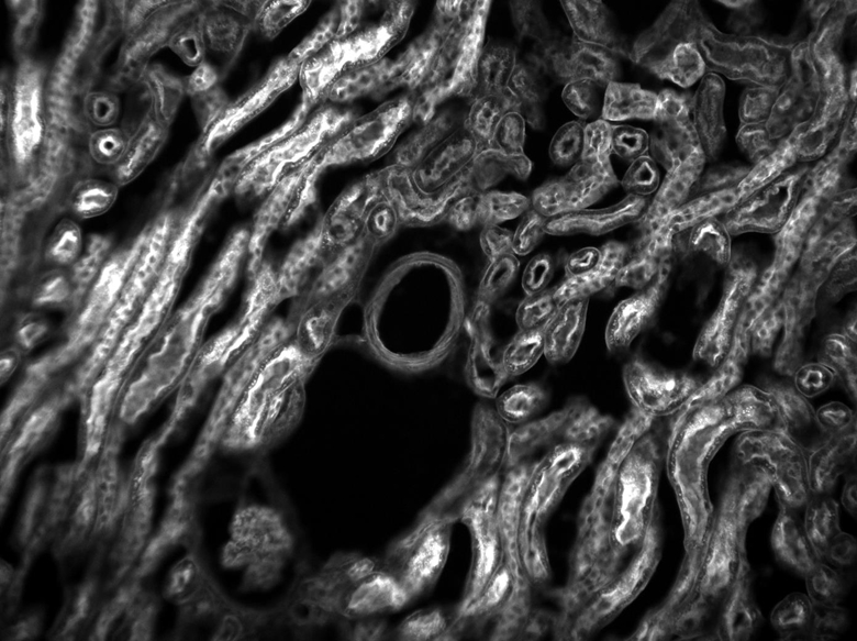
The images of a mouse kidney below were all acquired using the same objective and the same camera. However, the camera tubes used were different. Read from left to right, they demonstrate that decreasing the camera tube magnification enlarges the field of view at the expense of the size of the details in the image.

 Click to Enlarge
Figure 1: A Gaussian intensity profile only asymptotically approaches zero, so the spot size is defined by convention as either the full-width at half-maximum (FWHM) or 1/e2 value. We use the latter convention in this tutorial.
Spot Size Tutorial
The spot size achieved by focusing a laser beam with a lens or objective is an important parameter in many applications. This tutorial describes how the ratio of the initial beam diameter to the entrance pupil diameter, known as the truncation ratio, affects the focused spot size and provides expressions for calculating the spot size as a function of this ratio. Because the power transmitted by the focusing optic also depends upon the truncation ratio, the optimal balance between spot size and power transmission will depend upon the given application.
For each focusing objective that Thorlabs provides, we provide an estimate of the focused spot size when the incident Gaussian spot size (1/e2) is the same as the diameter of the entrance pupil. With this choice, the focused spot size is given by:
s ≈ 1.83λN, or equivalently, s ≈ 1.83λ/(2*NA), where NA is the numerical aperture of the objective; and the transmitted power is 86% of that of the incident beam.
Gaussian Beam Profile
Laser beams typically have a tranverse intensity profile that may be approximated by a Gaussian function,![]() ,
,
where w is the beam half-width or beam waist radius, conventionally defined as the radius (r) at which the intensity has decreased from its maximum axial value of I0 to I0/e2 ≈ 0.14I0. The spot size of a laser beam may be defined as twice the beam waist radius, and the corresponding circle with diameter equal to the spot size thus contains 86% of the beam's total intensity.
When a laser beam is focused by an objective, the resulting spot size (s) will depend upon the wavelength of the light (λ), the beam diameter as it enters the objective (S), the focal length of the objective (f), and the entrance pupil diameter of the objective (D). Dimensionless parameters are formed by taking the ratio of the focal length to the entrance pupil diameter and the ratio of the beam diameter to the entrance pupil diameter, which are known respectively as the f-number (N = f/D) and the truncation ratio (T = S/D). The f-number is fixed for a given objective, while the truncation ratio may be tuned by increasing or decreasing the incident beam diameter.
Spot Size vs. Truncation Ratio
The focused spot size is expressed in terms of the wavelength, truncation ratio, and f-number as
![]()
where K(T) is called the spot size coefficient and is a function of the truncation ratio [1]. In Figure 2 below, numerically computed values for K, obtained by calculating the focused intensity profile and extracting the focused spot size for discrete values of T, are plotted as black squares. As discussed in detail below, the solid-and-dashed blue line represents the coefficient predicted by Gaussian beam theory, the gray line represents the value of K for an Airy disk intensity profile, and the red line is a polynomial fit to the numerical values for T ≥ 0.5.
 Click to Enlarge
Figure 2: The shaded blue region below T < 0.5 indicates where Gaussian beam theory provides an accurate estimate of the focused spot size; however, above this value the effects of truncation cannot be neglected and the actual spot size is larger. As T → ∞, the coefficient approaches the Airy disk value of 1.6449 as indicated by the solid gray line.
 Click to Enlarge
Figure 3: The power transmitted through an entrance aperture of diameter D by a Gaussian beam with spot size S as a function of the truncation ratio T = S/D. The shaded blue region corresponds to the region where truncation effects on the spot size are negligible.
In both the large (T → ∞) and small (T → 0) limits, K approaches well-known theoretical results. For small T, which corresponds to an entrance pupil much larger than the Gaussian spot, K obeys the relation 1.27/T. This can be obtained from Gaussian beam propagation theory [2] which predicts that the minimum spot size a Gaussian beam can be focused to is s ≈ 1.27λf/S. By inserting factors of D to write this in terms of N and T, this expression can be cast into the same form as the spot size equation above, s = (1.27/T)λN, giving the result K = 1.27/T. As seen in Figure 2 above, this accurately predicts the focused spot size up to T ≈ 0.5, when the entrance pupil diameter D is twice as large as the spot size S. Above T = 0.5, it underestimates the value of K, as indicated by the deviation of the dashed blue line from the numerical results.
 Click to Enlarge
Figure 4: The spot size of an Airy disk profile is typically defined by the radius where the first intensity zero occurs. When the radius is expressed in units of λN, this corresponds to a radius of 1.22λN, or a spot size of 2.44λN. The 1/e2 radius for the same profile is 0.82245λN, or a spot size of 1.6449λN.
As T is increased, the illumination of the aperture becomes more and more uniform. The resulting intensity profile of the focused spot will therefore transition from a Gaussian profile to an Airy disk profile. In the large T limit, this is reflected in the value of K, which approaches a constant value of 1.6449 as T → ∞. This value corresponds to the 1/e2 spot size of an Airy disk instead of the better-known 2.44λN value which is where the first intensity minimum occurs, as shown in Figure 4 [3].
For intermediate values of T, which is the range in which most applications will fall, there is no exact theoretical result for K. Instead, the red line above represents a two-term polynomial fit to the numerical results, the coefficients of which are specified in the table below (the polynomial fit was performed using 1/T as the independent variable). This expression may be used to estimate K for T ≥ 0.5.
| Spot Size Coefficient, K(T) | |
|---|---|
| Truncation Ratio | Equation |
| T < 0.5 (Gaussian Regime) |
|
| T ≥ 0.5 (Intermediate and Uniform/Airy Regimes) |
|
Power Transmission and Spot Size
The results presented above suggest that, in the intermediate T regime, a smaller spot size may be achieved by increasing T. This, however, comes at the cost of reducing the overall power transmitted through the entrance aperture, and reductions in spot size may not be worth the loss in power. The power transmitted through an entrance pupil of diameter D as a function of T is plotted above in Figure 3. Already at T = 1, when the Gaussian spot size has the same diameter as the entrance pupil, the transmitted power is 86% of the incident power. By increasing T from 1 to 2, the spot size is reduced by only ≈ 9%, while the transmitted power decreases from 86% to 40%.
The optimal balance between spot size and power transmission will depend upon the given application. For each focusing objective that Thorlabs offers, we provide an estimate of the spot size using T = 1, when the Gaussian spot size is the same as the diameter of the entrance pupil. With this choice, the spot size is given by: s ≈ 1.83λN, or equivalently, s ≈ 1.83λ/(2*NA), where NA is the numerical aperture of the objective.
References
[1] Hakan Urey, "Spot size, depth-of-focus, and diffraction ring intensity formulas for truncated Gaussian beams," Appl. Opt. 43, 620-625 (2004)
[2] Sidney A. Self, "Focusing of spherical Gaussian beams," Appl. Opt. 22, 658-661 (1983)
[3] Eugene Hecht, "Optics," 4th Ed., Addison-Wesley (2002)
| Item # Suffix | Pulsed Damage Threshold |
|---|---|
| -UVB | 5.0 J/cm2 (355 nm, 10 ns, 20 Hz, Ø0.342 mm) |
| -NUV | 3.0 J/cm2 (355 nm, 6.6 ns, 20 Hz, Ø0.206 mm) |
| -266 | 5.0 J/cm2 (266 nm, 10 ns, 10 Hz, Ø0.127 mm) |
| -351 | 10 J/cm2 (355 nm, 10 ns, 10 Hz, Ø0.406 mm) |
Damage Threshold Data for High-Power Focusing Objectives AR Coatings
The limiting factor in the damage threshold for these objectives is their anti-reflection coating. The specifications to the right are measured data for the anti-reflection coatings deposited onto the optical surfaces of our high-power focusing objectives.
Laser Induced Damage Threshold Tutorial
The following is a general overview of how laser induced damage thresholds are measured and how the values may be utilized in determining the appropriateness of an optic for a given application. When choosing optics, it is important to understand the Laser Induced Damage Threshold (LIDT) of the optics being used. The LIDT for an optic greatly depends on the type of laser you are using. Continuous wave (CW) lasers typically cause damage from thermal effects (absorption either in the coating or in the substrate). Pulsed lasers, on the other hand, often strip electrons from the lattice structure of an optic before causing thermal damage. Note that the guideline presented here assumes room temperature operation and optics in new condition (i.e., within scratch-dig spec, surface free of contamination, etc.). Because dust or other particles on the surface of an optic can cause damage at lower thresholds, we recommend keeping surfaces clean and free of debris. For more information on cleaning optics, please see our Optics Cleaning tutorial.
Testing Method
Thorlabs' LIDT testing is done in compliance with ISO/DIS 11254 and ISO 21254 specifications.
First, a low-power/energy beam is directed to the optic under test. The optic is exposed in 10 locations to this laser beam for 30 seconds (CW) or for a number of pulses (pulse repetition frequency specified). After exposure, the optic is examined by a microscope (~100X magnification) for any visible damage. The number of locations that are damaged at a particular power/energy level is recorded. Next, the power/energy is either increased or decreased and the optic is exposed at 10 new locations. This process is repeated until damage is observed. The damage threshold is then assigned to be the highest power/energy that the optic can withstand without causing damage. A histogram such as that below represents the testing of one BB1-E02 mirror.
The photograph above is a protected aluminum-coated mirror after LIDT testing. In this particular test, it handled 0.43 J/cm2 (1064 nm, 10 ns pulse, 10 Hz, Ø1.000 mm) before damage.
| Example Test Data | |||
|---|---|---|---|
| Fluence | # of Tested Locations | Locations with Damage | Locations Without Damage |
| 1.50 J/cm2 | 10 | 0 | 10 |
| 1.75 J/cm2 | 10 | 0 | 10 |
| 2.00 J/cm2 | 10 | 0 | 10 |
| 2.25 J/cm2 | 10 | 1 | 9 |
| 3.00 J/cm2 | 10 | 1 | 9 |
| 5.00 J/cm2 | 10 | 9 | 1 |
According to the test, the damage threshold of the mirror was 2.00 J/cm2 (532 nm, 10 ns pulse, 10 Hz, Ø0.803 mm). Please keep in mind that these tests are performed on clean optics, as dirt and contamination can significantly lower the damage threshold of a component. While the test results are only representative of one coating run, Thorlabs specifies damage threshold values that account for coating variances.
Continuous Wave and Long-Pulse Lasers
When an optic is damaged by a continuous wave (CW) laser, it is usually due to the melting of the surface as a result of absorbing the laser's energy or damage to the optical coating (antireflection) [1]. Pulsed lasers with pulse lengths longer than 1 µs can be treated as CW lasers for LIDT discussions.
When pulse lengths are between 1 ns and 1 µs, laser-induced damage can occur either because of absorption or a dielectric breakdown (therefore, a user must check both CW and pulsed LIDT). Absorption is either due to an intrinsic property of the optic or due to surface irregularities; thus LIDT values are only valid for optics meeting or exceeding the surface quality specifications given by a manufacturer. While many optics can handle high power CW lasers, cemented (e.g., achromatic doublets) or highly absorptive (e.g., ND filters) optics tend to have lower CW damage thresholds. These lower thresholds are due to absorption or scattering in the cement or metal coating.

LIDT in linear power density vs. pulse length and spot size. For long pulses to CW, linear power density becomes a constant with spot size. This graph was obtained from [1].
Pulsed lasers with high pulse repetition frequencies (PRF) may behave similarly to CW beams. Unfortunately, this is highly dependent on factors such as absorption and thermal diffusivity, so there is no reliable method for determining when a high PRF laser will damage an optic due to thermal effects. For beams with a high PRF both the average and peak powers must be compared to the equivalent CW power. Additionally, for highly transparent materials, there is little to no drop in the LIDT with increasing PRF.
In order to use the specified CW damage threshold of an optic, it is necessary to know the following:
- Wavelength of your laser
- Beam diameter of your beam (1/e2)
- Approximate intensity profile of your beam (e.g., Gaussian)
- Linear power density of your beam (total power divided by 1/e2 beam diameter)
Thorlabs expresses LIDT for CW lasers as a linear power density measured in W/cm. In this regime, the LIDT given as a linear power density can be applied to any beam diameter; one does not need to compute an adjusted LIDT to adjust for changes in spot size, as demonstrated by the graph to the right. Average linear power density can be calculated using the equation below.
The calculation above assumes a uniform beam intensity profile. You must now consider hotspots in the beam or other non-uniform intensity profiles and roughly calculate a maximum power density. For reference, a Gaussian beam typically has a maximum power density that is twice that of the uniform beam (see lower right).
Now compare the maximum power density to that which is specified as the LIDT for the optic. If the optic was tested at a wavelength other than your operating wavelength, the damage threshold must be scaled appropriately. A good rule of thumb is that the damage threshold has a linear relationship with wavelength such that as you move to shorter wavelengths, the damage threshold decreases (i.e., a LIDT of 10 W/cm at 1310 nm scales to 5 W/cm at 655 nm):
While this rule of thumb provides a general trend, it is not a quantitative analysis of LIDT vs wavelength. In CW applications, for instance, damage scales more strongly with absorption in the coating and substrate, which does not necessarily scale well with wavelength. While the above procedure provides a good rule of thumb for LIDT values, please contact Tech Support if your wavelength is different from the specified LIDT wavelength. If your power density is less than the adjusted LIDT of the optic, then the optic should work for your application.
Please note that we have a buffer built in between the specified damage thresholds online and the tests which we have done, which accommodates variation between batches. Upon request, we can provide individual test information and a testing certificate. The damage analysis will be carried out on a similar optic (customer's optic will not be damaged). Testing may result in additional costs or lead times. Contact Tech Support for more information.
Pulsed Lasers
As previously stated, pulsed lasers typically induce a different type of damage to the optic than CW lasers. Pulsed lasers often do not heat the optic enough to damage it; instead, pulsed lasers produce strong electric fields capable of inducing dielectric breakdown in the material. Unfortunately, it can be very difficult to compare the LIDT specification of an optic to your laser. There are multiple regimes in which a pulsed laser can damage an optic and this is based on the laser's pulse length. The highlighted columns in the table below outline the relevant pulse lengths for our specified LIDT values.
Pulses shorter than 10-9 s cannot be compared to our specified LIDT values with much reliability. In this ultra-short-pulse regime various mechanics, such as multiphoton-avalanche ionization, take over as the predominate damage mechanism [2]. In contrast, pulses between 10-7 s and 10-4 s may cause damage to an optic either because of dielectric breakdown or thermal effects. This means that both CW and pulsed damage thresholds must be compared to the laser beam to determine whether the optic is suitable for your application.
| Pulse Duration | t < 10-9 s | 10-9 < t < 10-7 s | 10-7 < t < 10-4 s | t > 10-4 s |
|---|---|---|---|---|
| Damage Mechanism | Avalanche Ionization | Dielectric Breakdown | Dielectric Breakdown or Thermal | Thermal |
| Relevant Damage Specification | No Comparison (See Above) | Pulsed | Pulsed and CW | CW |
When comparing an LIDT specified for a pulsed laser to your laser, it is essential to know the following:
LIDT in energy density vs. pulse length and spot size. For short pulses, energy density becomes a constant with spot size. This graph was obtained from [1].
- Wavelength of your laser
- Energy density of your beam (total energy divided by 1/e2 area)
- Pulse length of your laser
- Pulse repetition frequency (prf) of your laser
- Beam diameter of your laser (1/e2 )
- Approximate intensity profile of your beam (e.g., Gaussian)
The energy density of your beam should be calculated in terms of J/cm2. The graph to the right shows why expressing the LIDT as an energy density provides the best metric for short pulse sources. In this regime, the LIDT given as an energy density can be applied to any beam diameter; one does not need to compute an adjusted LIDT to adjust for changes in spot size. This calculation assumes a uniform beam intensity profile. You must now adjust this energy density to account for hotspots or other nonuniform intensity profiles and roughly calculate a maximum energy density. For reference a Gaussian beam typically has a maximum energy density that is twice that of the 1/e2 beam.
Now compare the maximum energy density to that which is specified as the LIDT for the optic. If the optic was tested at a wavelength other than your operating wavelength, the damage threshold must be scaled appropriately [3]. A good rule of thumb is that the damage threshold has an inverse square root relationship with wavelength such that as you move to shorter wavelengths, the damage threshold decreases (i.e., a LIDT of 1 J/cm2 at 1064 nm scales to 0.7 J/cm2 at 532 nm):
You now have a wavelength-adjusted energy density, which you will use in the following step.
Beam diameter is also important to know when comparing damage thresholds. While the LIDT, when expressed in units of J/cm², scales independently of spot size; large beam sizes are more likely to illuminate a larger number of defects which can lead to greater variances in the LIDT [4]. For data presented here, a <1 mm beam size was used to measure the LIDT. For beams sizes greater than 5 mm, the LIDT (J/cm2) will not scale independently of beam diameter due to the larger size beam exposing more defects.
The pulse length must now be compensated for. The longer the pulse duration, the more energy the optic can handle. For pulse widths between 1 - 100 ns, an approximation is as follows:
Use this formula to calculate the Adjusted LIDT for an optic based on your pulse length. If your maximum energy density is less than this adjusted LIDT maximum energy density, then the optic should be suitable for your application. Keep in mind that this calculation is only used for pulses between 10-9 s and 10-7 s. For pulses between 10-7 s and 10-4 s, the CW LIDT must also be checked before deeming the optic appropriate for your application.
Please note that we have a buffer built in between the specified damage thresholds online and the tests which we have done, which accommodates variation between batches. Upon request, we can provide individual test information and a testing certificate. Contact Tech Support for more information.
[1] R. M. Wood, Optics and Laser Tech. 29, 517 (1998).
[2] Roger M. Wood, Laser-Induced Damage of Optical Materials (Institute of Physics Publishing, Philadelphia, PA, 2003).
[3] C. W. Carr et al., Phys. Rev. Lett. 91, 127402 (2003).
[4] N. Bloembergen, Appl. Opt. 12, 661 (1973).

In order to illustrate the process of determining whether a given laser system will damage an optic, a number of example calculations of laser induced damage threshold are given below. For assistance with performing similar calculations, we provide a spreadsheet calculator that can be downloaded by clicking the button to the right. To use the calculator, enter the specified LIDT value of the optic under consideration and the relevant parameters of your laser system in the green boxes. The spreadsheet will then calculate a linear power density for CW and pulsed systems, as well as an energy density value for pulsed systems. These values are used to calculate adjusted, scaled LIDT values for the optics based on accepted scaling laws. This calculator assumes a Gaussian beam profile, so a correction factor must be introduced for other beam shapes (uniform, etc.). The LIDT scaling laws are determined from empirical relationships; their accuracy is not guaranteed. Remember that absorption by optics or coatings can significantly reduce LIDT in some spectral regions. These LIDT values are not valid for ultrashort pulses less than one nanosecond in duration.
A Gaussian beam profile has about twice the maximum intensity of a uniform beam profile.
CW Laser Example
Suppose that a CW laser system at 1319 nm produces a 0.5 W Gaussian beam that has a 1/e2 diameter of 10 mm. A naive calculation of the average linear power density of this beam would yield a value of 0.5 W/cm, given by the total power divided by the beam diameter:
However, the maximum power density of a Gaussian beam is about twice the maximum power density of a uniform beam, as shown in the graph to the right. Therefore, a more accurate determination of the maximum linear power density of the system is 1 W/cm.
An AC127-030-C achromatic doublet lens has a specified CW LIDT of 350 W/cm, as tested at 1550 nm. CW damage threshold values typically scale directly with the wavelength of the laser source, so this yields an adjusted LIDT value:
The adjusted LIDT value of 350 W/cm x (1319 nm / 1550 nm) = 298 W/cm is significantly higher than the calculated maximum linear power density of the laser system, so it would be safe to use this doublet lens for this application.
Pulsed Nanosecond Laser Example: Scaling for Different Pulse Durations
Suppose that a pulsed Nd:YAG laser system is frequency tripled to produce a 10 Hz output, consisting of 2 ns output pulses at 355 nm, each with 1 J of energy, in a Gaussian beam with a 1.9 cm beam diameter (1/e2). The average energy density of each pulse is found by dividing the pulse energy by the beam area:
As described above, the maximum energy density of a Gaussian beam is about twice the average energy density. So, the maximum energy density of this beam is ~0.7 J/cm2.
The energy density of the beam can be compared to the LIDT values of 1 J/cm2 and 3.5 J/cm2 for a BB1-E01 broadband dielectric mirror and an NB1-K08 Nd:YAG laser line mirror, respectively. Both of these LIDT values, while measured at 355 nm, were determined with a 10 ns pulsed laser at 10 Hz. Therefore, an adjustment must be applied for the shorter pulse duration of the system under consideration. As described on the previous tab, LIDT values in the nanosecond pulse regime scale with the square root of the laser pulse duration:
This adjustment factor results in LIDT values of 0.45 J/cm2 for the BB1-E01 broadband mirror and 1.6 J/cm2 for the Nd:YAG laser line mirror, which are to be compared with the 0.7 J/cm2 maximum energy density of the beam. While the broadband mirror would likely be damaged by the laser, the more specialized laser line mirror is appropriate for use with this system.
Pulsed Nanosecond Laser Example: Scaling for Different Wavelengths
Suppose that a pulsed laser system emits 10 ns pulses at 2.5 Hz, each with 100 mJ of energy at 1064 nm in a 16 mm diameter beam (1/e2) that must be attenuated with a neutral density filter. For a Gaussian output, these specifications result in a maximum energy density of 0.1 J/cm2. The damage threshold of an NDUV10A Ø25 mm, OD 1.0, reflective neutral density filter is 0.05 J/cm2 for 10 ns pulses at 355 nm, while the damage threshold of the similar NE10A absorptive filter is 10 J/cm2 for 10 ns pulses at 532 nm. As described on the previous tab, the LIDT value of an optic scales with the square root of the wavelength in the nanosecond pulse regime:
This scaling gives adjusted LIDT values of 0.08 J/cm2 for the reflective filter and 14 J/cm2 for the absorptive filter. In this case, the absorptive filter is the best choice in order to avoid optical damage.
Pulsed Microsecond Laser Example
Consider a laser system that produces 1 µs pulses, each containing 150 µJ of energy at a repetition rate of 50 kHz, resulting in a relatively high duty cycle of 5%. This system falls somewhere between the regimes of CW and pulsed laser induced damage, and could potentially damage an optic by mechanisms associated with either regime. As a result, both CW and pulsed LIDT values must be compared to the properties of the laser system to ensure safe operation.
If this relatively long-pulse laser emits a Gaussian 12.7 mm diameter beam (1/e2) at 980 nm, then the resulting output has a linear power density of 5.9 W/cm and an energy density of 1.2 x 10⁻⁴ J/cm2 per pulse. This can be compared to the LIDT values for a WPQ10E-980 polymer zero-order quarter-wave plate, which are 5 W/cm for CW radiation at 810 nm and 5 J/cm2 for a 10 ns pulse at 810 nm. As before, the CW LIDT of the optic scales linearly with the laser wavelength, resulting in an adjusted CW value of 6 W/cm at 980 nm. On the other hand, the pulsed LIDT scales with the square root of the laser wavelength and the square root of the pulse duration, resulting in an adjusted value of 55 J/cm2 for a 1 µs pulse at 980 nm. The pulsed LIDT of the optic is significantly greater than the energy density of the laser pulse, so individual pulses will not damage the wave plate. However, the large average linear power density of the laser system may cause thermal damage to the optic, much like a high-power CW beam.
Laser Safety and Classification
Safe practices and proper usage of safety equipment should be taken into consideration when operating lasers. The eye is susceptible to injury, even from very low levels of laser light. Thorlabs offers a range of laser safety accessories that can be used to reduce the risk of accidents or injuries. Laser emission in the visible and near infrared spectral ranges has the greatest potential for retinal injury, as the cornea and lens are transparent to those wavelengths, and the lens can focus the laser energy onto the retina.
 |
 |
 |
 |
 |
 |
 |
 |
 |
Safe Practices and Light Safety Accessories
- Laser safety eyewear must be worn whenever working with Class 3 or 4 lasers.
- Regardless of laser class, Thorlabs recommends the use of laser safety eyewear whenever working with laser beams with non-negligible powers, since metallic tools such as screwdrivers can accidentally redirect a beam.
- Laser goggles designed for specific wavelengths should be clearly available near laser setups to protect the wearer from unintentional laser reflections.
- Goggles are marked with the wavelength range over which protection is afforded and the minimum optical density within that range.
- Laser Safety Curtains and Laser Safety Fabric shield other parts of the lab from high energy lasers.
- Blackout Materials can prevent direct or reflected light from leaving the experimental setup area.
- Thorlabs' Enclosure Systems can be used to contain optical setups to isolate or minimize laser hazards.
- A fiber-pigtailed laser should always be turned off before connecting it to or disconnecting it from another fiber, especially when the laser is at power levels above 10 mW.
- All beams should be terminated at the edge of the table, and laboratory doors should be closed whenever a laser is in use.
- Do not place laser beams at eye level.
- Carry out experiments on an optical table such that all laser beams travel horizontally.
- Remove unnecessary reflective items such as reflective jewelry (e.g., rings, watches, etc.) while working near the beam path.
- Be aware that lenses and other optical devices may reflect a portion of the incident beam from the front or rear surface.
- Operate a laser at the minimum power necessary for any operation.
- If possible, reduce the output power of a laser during alignment procedures.
- Use beam shutters and filters to reduce the beam power.
- Post appropriate warning signs or labels near laser setups or rooms.
- Use a laser sign with a lightbox if operating Class 3R or 4 lasers (i.e., lasers requiring the use of a safety interlock).
- Do not use Laser Viewing Cards in place of a proper Beam Trap.
Laser Classification
Lasers are categorized into different classes according to their ability to cause eye and other damage. The International Electrotechnical Commission (IEC) is a global organization that prepares and publishes international standards for all electrical, electronic, and related technologies. The IEC document 60825-1 outlines the safety of laser products. A description of each class of laser is given below:
| Class | Description | Warning Label |
|---|---|---|
| 1 | This class of laser is safe under all conditions of normal use, including use with optical instruments for intrabeam viewing. Lasers in this class do not emit radiation at levels that may cause injury during normal operation, and therefore the maximum permissible exposure (MPE) cannot be exceeded. Class 1 lasers can also include enclosed, high-power lasers where exposure to the radiation is not possible without opening or shutting down the laser. |  |
| 1M | Class 1M lasers are safe except when used in conjunction with optical components such as telescopes and microscopes. Lasers belonging to this class emit large-diameter or divergent beams, and the MPE cannot normally be exceeded unless focusing or imaging optics are used to narrow the beam. However, if the beam is refocused, the hazard may be increased and the class may be changed accordingly. |  |
| 2 | Class 2 lasers, which are limited to 1 mW of visible continuous-wave radiation, are safe because the blink reflex will limit the exposure in the eye to 0.25 seconds. This category only applies to visible radiation (400 - 700 nm). |  |
| 2M | Because of the blink reflex, this class of laser is classified as safe as long as the beam is not viewed through optical instruments. This laser class also applies to larger-diameter or diverging laser beams. |  |
| 3R | Class 3R lasers produce visible and invisible light that is hazardous under direct and specular-reflection viewing conditions. Eye injuries may occur if you directly view the beam, especially when using optical instruments. Lasers in this class are considered safe as long as they are handled with restricted beam viewing. The MPE can be exceeded with this class of laser; however, this presents a low risk level to injury. Visible, continuous-wave lasers in this class are limited to 5 mW of output power. |  |
| 3B | Class 3B lasers are hazardous to the eye if exposed directly. Diffuse reflections are usually not harmful, but may be when using higher-power Class 3B lasers. Safe handling of devices in this class includes wearing protective eyewear where direct viewing of the laser beam may occur. Lasers of this class must be equipped with a key switch and a safety interlock; moreover, laser safety signs should be used, such that the laser cannot be used without the safety light turning on. Laser products with power output near the upper range of Class 3B may also cause skin burns. |  |
| 4 | This class of laser may cause damage to the skin, and also to the eye, even from the viewing of diffuse reflections. These hazards may also apply to indirect or non-specular reflections of the beam, even from apparently matte surfaces. Great care must be taken when handling these lasers. They also represent a fire risk, because they may ignite combustible material. Class 4 lasers must be equipped with a key switch and a safety interlock. |  |
| All class 2 lasers (and higher) must display, in addition to the corresponding sign above, this triangular warning sign. |  |
|
| Posted Comments: | |
Ori Golani
(posted 2022-02-22 19:45:53.777) Can you please provide the transmission and focal shift for LMU-5X-NUV and LMU-20X-NUV at 1030nm wavelength?
Is the power loss caused due to absorption, or simply reflection? cdolbashian
(posted 2022-03-08 11:13:13.0) Thank you for reaching out to us Ori. I have contacted you directly to discuss the focal shift and theoretical transmission at the specified wavelength. The power losses are mainly due to reflection of the -NUV coating. user
(posted 2021-11-16 10:56:12.24) What is the tolerance on parafocal length of LMU-5X-NUV (63.8 mm) ? YLohia
(posted 2021-11-23 02:04:47.0) Thank you for contacting Thorlabs. I have reached out to you directly with this information. Paul Godijn
(posted 2021-04-22 04:56:05.033) Best sales
Can you give me the spot size,
I want to build an installation that can detect cut lines in a coating.
With a linear slide I let this laser move over the surface.
That way I can measure the mutual distance of these cuts.
The linear carriage to be used has a displacement accuracy of +/- 2 mu The cut itself is +/- 260 microns wide and I am supposed to be able to locate the deepest point.
Thank you in advance,
Sincerely,
Paul Godijn.
Paul.Godijn@MacdermidAlpha.com YLohia
(posted 2021-04-22 11:25:26.0) Hello Paul, thank you for contacting Thorlabs. Please see the specs table below. We specify the focused spot size for the LMUL-50X-UVB to be 0.7 µm at the center wavelength, assuming the entrance aperture is filled and the input beam profile is Gaussian. Jhon Vera
(posted 2021-01-25 21:51:43.943) Hello, we want to use the LMU-15X-UVB for a 4 W power appliction. The described transmission is around ~90% for the 343 nm wavelength. Will the other ~10 % be absorbed by the AR coating? Do you have some kind of thermal effect measurement or absorption measurement? YLohia
(posted 2021-01-28 10:39:50.0) Hello, thank you for contacting Thorlabs. Losses in the LMU-15X-UVB are distributed over multiple optical surfaces and the losses mostly come from surface reflections, so thermal effects of absorption can be neglected. Unfortunately, we don't have any thermal effect measurements for this objective lens. d00245003
(posted 2018-10-14 00:06:47.433) Is it possible to use the LMU-15X-193 in the vacuum environment (~5e-6 Torr) YLohia
(posted 2018-10-15 12:00:38.0) Hello, unfortunately, the LMU-15X-193 is not recommended for vacuum use. We may be able to offer a special vacuum compatible version of this depending on your requirements. We will reach out to you directly to discuss this. jasmine.sears
(posted 2018-02-26 18:39:10.123) What is the back focal distance of the LMU-20X-NUV objective? llamb
(posted 2018-04-05 09:16:24.0) Thank you for contacting Thorlabs. Could you please clarify what you mean by the back focal distance? The back focal length is usually specified from the last lens surface, which is inside the objective housing in this case. If you are looking for the parfocal length (the distance from the mounting surface to the focus), this is 39.1 mm for the LMU-20X-NUV. I have reached out to you directly as well. dominik
(posted 2016-07-14 21:16:31.887) Can I get a 40x objective with a narrow band pass filter at around 213? What coating are available for the 40x ones leo.basset
(posted 2016-05-24 08:16:35.057) Is it possible to use these for imaging applications or are they limited to focusing light? besembeson
(posted 2016-05-25 12:20:32.0) Response from Bweh at Thorlabs USA: These are designed for focusing applications, which will typically be for high power monochromatic sources. Except your imaging application is with a monochromatic source at the design wavelength, the image will suffer from spherical and chromatic aberrations. I will recommend considering the other objectives we provide designed for general imaging applications. hussainm1
(posted 2016-03-15 12:39:57.987) What is the transmittance of both broadband and narrowband 20x objective at wavelength range 800-900 nm? besembeson
(posted 2016-03-17 11:21:44.0) Response from Bweh at Thorlabs USA: I will contact you with an estimate. user
(posted 2015-08-02 16:29:58.373) what is the thread of those? myanakas
(posted 2015-08-03 10:03:51.0) Response from Mike at Thorlabs: Thank you for your feedback. Each of our High-Power UV Focusing Objectives have an externally RMS-threaded (0.800"-36) Housing. Since contact information was not provided I was unable to contact you directly. If you are in need of further assistance please contact our technical support department at TechSupport@Thorlabs.com user
(posted 2014-05-07 09:47:49.857) What is focus length of tube lens if considering magnifications? 200mm ? 180mm? jlow
(posted 2014-05-07 11:33:04.0) Response from Jeremy at Thorlabs: The tube lens focal length is 200mm. klee
(posted 2009-10-15 10:23:07.0) A response from Ken at Thorlabs to cjohansson: The link is working now. cjohansson
(posted 2009-10-15 09:26:27.0) the link to "visible imaging objectives" in the selection guide is broken. |

 Zoom
Zoom- AR Coated for 240 - 360 nm
- 10X, 20X, or 50X Magnification
- Diffraction-Limited Performance
- 0.25, 0.36, or 0.42 Numerical Aperture
- External W26 x 0.706 Threads, 5 mm Depth
These objectives provide long working distances while keeping axial focal shift low. Their optical design is chromatically optimized in the UV wavelength range. Diffraction-limited performance is guaranteed over the entire clear aperture. These objectives are ideal for laser cutting, surgical laser focusing, and spectrometry applications. They can also be used for scanning and micro-imaging applications like brightfield imaging under narrowband, UV laser illumination. Each objective is shipped in an objective case comprised of an OC2M26 lid and an OC24 canister. Custom AR Coatings can be requested by contacting Tech Support; options include broadband NUV (325 nm - 500 nm), dual band (266 and 532 nm), and laser line (248 nm, 266 nm, 355 nm, or 532 nm). Please see the Graphs tab for more details.
| Item # | AR Coating Range |
Ma | WD | EFL | PFL | NA | EPb | Spot Sizec | OFN | Typical Transmission |
Max Reflectance per Surfaced |
Pulsed Damage Threshold |
Design Tube Lens Focal Lengthe |
|---|---|---|---|---|---|---|---|---|---|---|---|---|---|
| LMUL-10X-UVB | 240 - 360 nm | 10X | 20.0 mm | 20 mm | 95.0 mm | 0.25 | 10.0 mm | 1.3 µm | 24 | Raw Data |
(240 - 360 nm) |
5.0 J/cm2 (355 nm, 10 ns, 20 Hz, Ø0.342 mm) |
200 mm |
| LMUL-20X-UVB | 20X | 15.3 mm | 10 mm | 0.36 | 7.2 mm | 0.9 µm | Raw Data |
||||||
| LMUL-50X-UVB | 50X | 12.0 mm | 4 mm | 0.42 | 3.4 mm | 0.8 µm | Raw Data |

 Zoom
Zoom
Click to Enlarge
Click Here for Raw Data
- AR Coated for 240 - 360 nm or 325 - 500 nm
- 5X, 20X, or 40X Magnification Available
- Diffraction-Limited Performance for Beam Diameters ≤70% of Clear Aperture
- Numerical Apertures from 0.12 to 0.49
- External RMS (0.800"-36) Threads, 3.8 mm Depth
These 5X, 20X, and 40X objectives are chromatically corrected to minimize the axial focal shift across the AR coating wavelength range. Diffraction-limited performance can be achieved with beam diameters ≤70% of each objective's clear aperture. These objectives are ideal for focusing or collecting polychromatic light, making them well suited for use in spectrometry, wafer inspection, or surgical laser applications. Their small field of view limits their performance in imaging applications.
The external RMS (0.800"-36) threads allow these objectives to be mounted to our fiber launch systems or to any of our flexure stages using a HCS013 RMS mount. An objective case (OC2RMS lid and OC22 canister) and aluminum cap (RMSCP1) are available for purchase separately.
| Item # | AR Coating Range |
Ma | WD | EFL | PFL | NA | EPb | Spot Sizec | OFN | Typical Transmission |
Max Reflectance per Surfaced |
Pulsed Damage Threshold |
Design Tube Lens Focal Lengthe |
|---|---|---|---|---|---|---|---|---|---|---|---|---|---|
| LMU-5X-UVB | 240 - 360 nm | 5X | 37.3 mm | 39.8 mm | 63.7 mm | 0.12 | 9.9 mm | 3 µm | 18 | Raw Data |
<1.5% (240 - 360 nm) |
5.0 J/cm2 (355 nm, 10 ns, 20 Hz, Ø0.342 mm) |
200 mm |
| LMU-5X-NUV | 325 - 500 nm | 5X | 37.5 mm | 39.9 mm | 63.8 mm | 0.12 | 9.9 mm | 4 µm | 18 | Raw Data |
<1.0% (325 - 500 nm) |
3.0 J/cm2 (355 nm, 6.6 ns, 20 Hz, Ø0.206 mm) |
|
| LMU-20X-UVB | 240 - 360 nm | 20X | 4.1 mm | 9.9 mm | 39.1 mm | 0.39 | 8.0 mm | 1 µm | 5 | Raw Data |
<1.5% (240 - 360 nm) |
5.0 J/cm2 (355 nm, 10 ns, 20 Hz, Ø0.342 mm) |
|
| LMU-20X-NUV | 325 - 500 nm | 20X | 4.1 mm | 10.1 mm | 39.1 mm | 0.38 | 8.0 mm | 1 µm | 5 | Raw Data |
<1.0% (325 - 500 nm) |
3.0 J/cm2 (355 nm, 6.6 ns, 20 Hz, Ø0.206 mm) |
|
| LMU-40X-UVB | 240 - 360 nm | 40X | 0.8 mm | 5.2 mm | 34.4 mm | 0.49 | 5.1 mm | 1 µm | 10 | Raw Data |
<1.5% (240 - 360 nm) |
5.0 J/cm2 (355 nm, 10 ns, 20 Hz, Ø0.342 mm) |
|
| LMU-40X-NUV | 325 - 500 nm | 40X | 0.8 mm | 5.3 mm | 34.5 mm | 0.47 | 5.1 mm | 1 µm | 10 | Raw Data |
<1.0% (325 - 500 nm) |
3.0 J/cm2 (355 nm, 6.6 ns, 20 Hz, Ø0.206 mm) |

 Zoom
Zoom
Click to Enlarge
Click Here for Raw Data
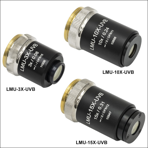
- AR Coated for 240 - 360 nm or 325 - 500 nm
- 3X, 10X, or 15X Magnification Available
- Diffraction-Limited Performance for Beam Diameters ≤70% of Clear Aperture
- Numerical Apertures from 0.08 to 0.31
- External RMS (0.800"-36) Threads, 3.8 mm Depth
These objectives offer 3X, 10X, and 15X magnification. Due to their monochromatic optical design, a narrow-bandwidth laser within the AR coating wavelength range should be used to achieve optimal optical performance. Diffraction-limited performance can be achieved with beam diameters ≤70% of each objective's clear aperture. We also offer narrowband-coated versions of these objectives below.
The external RMS (0.800"-36) threads allow these objectives to be mounted to our fiber launch systems or to any of our flexure stages using a HCS013 RMS mount. An objective case (OC2RMS lid and OC22 canister) and aluminum cap (RMSCP1) are available for purchase separately
| Item # | AR Coating Range |
Ma | WD | EFL | PFL | NA | EPb | Spot Sizec | OFN | Typical Transmission |
Max Reflectance per Surfaced |
Pulsed Damage Threshold |
Design Tube Lens Focal Lengthe |
|---|---|---|---|---|---|---|---|---|---|---|---|---|---|
| LMU-3X-UVB | 240 - 360 nm | 3X | 50.1 mm | 60.4 mm | 76.3 mm | 0.08 | 9.9 mm | 4 µm | 15 | Raw Data |
<1.5% (240 - 360 nm) |
5.0 J/cm2 (355 nm, 10 ns, 20 Hz, Ø0.342 mm) |
200 mm |
| LMU-3X-NUV | 325 - 500 nm | 3X | 50.7 mm | 61.0 mm | 76.9 mm | 0.08 | 9.9 mm | 6 µm | 17 | Raw Data |
<1.0% (325 - 500 nm) |
3.0 J/cm2 (355 nm, 6.6 ns, 20 Hz, Ø0.206 mm) |
|
| LMU-10X-UVB | 240 - 360 nm | 10X | 15.0 mm | 20.5 mm | 47.2 mm | 0.24 | 9.9 mm | 2 µm | 11 | Raw Data |
<1.5% (240 - 360 nm) |
5.0 J/cm2 (355 nm, 10 ns, 20 Hz, Ø0.342 mm) |
|
| LMU-10X-NUV | 325 - 500 nm | 10X | 15.6 mm | 21.2 mm | 47.7 mm | 0.23 | 9.9 mm | 1 µm | 13 | Raw Data |
<1.0% (325 - 500 nm) |
3.0 J/cm2 (355 nm, 6.6 ns, 20 Hz, Ø0.206 mm) |
|
| LMU-15X-UVB | 240 - 360 nm | 15X | 8.3 mm | 13.6 mm | 44.7 mm | 0.31 | 8.5 mm | 1 µm | 12 | Raw Data |
<1.5% (240 - 360 nm) |
5.0 J/cm2 (355 nm, 10 ns, 20 Hz, Ø0.342 mm) |
|
| LMU-15X-NUV | 325 - 500 nm | 15X | 8.6 mm | 14.1 mm | 45.1 mm | 0.30 | 8.5 mm | 2 µm | 13 | Raw Data |
<1.0% (325 - 500 nm) |
3.0 J/cm2 (355 nm, 6.6 ns, 20 Hz, Ø0.206 mm) |

 Zoom
Zoom
Click to Enlarge
Click Here for Raw Data
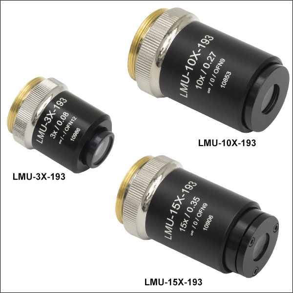
- AR Coated for 192 - 194 nm, 240 - 260 nm, 248 - 287 nm, or 325 - 380 nm
- 3X, 10X, or 15X Magnification Available
- Diffraction-Limited Performance for Beam Diameters ≤70% of Clear Aperture
- Numerical Apertures from 0.08 to 0.35
- External RMS (0.800"-36) Threads, 3.8 mm Depth
These 3X, 10X, and 15X objectives are treated with narrowband AR coatings centered around Excimer laser lines with <1% maximum reflectance per surface and high damage thresholds, making them ideal for laser cutting and micromachining components at high powers.
The external RMS (0.800"-36) threads allow these objectives to be mounted to our fiber launch systems or to any of our flexure stages using a HCS013 RMS mount. An objective case (OC2RMS lid and OC22 canister) and aluminum cap (RMSCP1) are available for purchase separately.
| Item # | AR Coating Range |
Ma | WD | EFL | PFL | NA | EPb | Spot Sizec | OFN | Typical Transmission |
Max Reflectance per Surfaced |
Pulsed Damage Threshold |
Design Tube Lens Focal Lengthe |
|---|---|---|---|---|---|---|---|---|---|---|---|---|---|
| LMU-3X-193 | 192 - 194 nm | 3X | 48.6 mm | 59.0 mm | 74.7 mm | 0.08 | 9.9 mm | 2 µm | 12 | Raw Data |
<0.3% (192 - 194 nm) | - | 200 mm |
| LMU-3X-248 | 240 - 260 nm | 3X | 49.5 mm | 59.8 mm | 75.7 mm | 0.08 | 9.9 mm | 3 µm | 15 | Raw Data |
<0.5% (240 - 260 nm) | - | |
| LMU-3X-266 | 248 - 287 nm | 3X | 49.7 mm | 60.0 mm | 75.9 mm | 0.08 | 9.9 mm | 3 µm | 16 | Raw Data |
<0.7% (248 - 287 nm) <0.2% (256 - 275 nm) |
5.0 J/cm2 (266 nm, 10 ns, 10 Hz, Ø0.127 mm) |
|
| LMU-3X-351 | 325 - 380 nm | 3X | 50.5 mm | 60.7 mm | 76.6 mm | 0.08 | 9.9 mm | 4 µm | 18 | Raw Data |
<0.7% (325 - 380 nm) <0.2% (335 - 362 nm) |
10 J/cm2 (355 nm, 10 ns, 10 Hz, Ø0.406 mm) |
|
| LMU-10X-193 | 192 - 194 nm | 10X | 13.2 mm | 18.2 mm | 45.3 mm | 0.27 | 9.9 mm | 1 µm | 9 | Raw Data |
<0.3% (192 - 194 nm) | - | |
| LMU-10X-248 | 240 - 260 nm | 10X | 14.5 mm | 19.8 mm | 46.6 mm | 0.25 | 9.9 mm | 1 µm | 11 | Raw Data |
<0.5% (240 - 260 nm) | - | |
| LMU-10X-266 | 248 - 287 nm | 10X | 14.7 mm | 20.1 mm | 46.8 mm | 0.25 | 9.9 mm | 1 µm | 12 | Raw Data |
<0.7% (248 - 287 nm) <0.2% (256 - 275 nm) |
5.0 J/cm2 (266 nm, 10 ns, 10 Hz, Ø0.127 mm) |
|
| LMU-10X-351 | 325 - 380 nm | 10X | 15.4 mm | 20.9 mm | 47.5 mm | 0.24 | 9.9 mm | 1 µm | 14 | Raw Data |
<0.7% (325 - 380 nm) <0.2% (335 - 362 nm) |
10 J/cm2 (355 nm, 10 ns, 10 Hz, Ø0.406 mm) |
|
| LMU-15X-193 | 192 - 194 nm | 15X | 7.2 mm | 12.0 mm | 43.7 mm | 0.35 | 8.5 mm | 1 µm | 9 | Raw Data |
<0.3% (192 - 194 nm) | - | |
| LMU-15X-248 | 240 - 260 nm | 15X | 8.0 mm | 13.1 mm | 44.4 mm | 0.32 | 8.5 mm | 1 µm | 12 | Raw Data |
<0.5% (240 - 260 nm) | - | |
| LMU-15X-266 | 248 - 287 nm | 15X | 8.1 mm | 13.3 mm | 44.5 mm | 0.32 | 8.5 mm | 1 µm | 13 | Raw Data |
<0.7% (248 - 287 nm) <0.2% (256 - 275 nm) |
5.0 J/cm2 (266 nm, 10 ns, 10 Hz, Ø0.127 mm) |
|
| LMU-15X-351 | 325 - 380 nm | 15X | 8.5 mm | 13.9 mm | 44.9 mm | 0.31 | 8.5 mm | 1 µm | 13 | Raw Data |
<0.7% (325 - 380 nm) <0.2% (335 - 362 nm) |
10 J/cm2 (355 nm, 10 ns, 10 Hz, Ø0.406 mm) |