 Products Home / Optical Systems / Objective Lenses, Scan Lenses, and Tube Lenses / Reflective Microscope Objectives
Reflective Microscope Objectives
- Diffraction-Limited Performance and No Chromatic Aberration
- 15X, 25X, or 40X Magnification
- Infinity-Corrected or 160 mm Back Focal Length
- UV-Enhanced Aluminum and Protected Silver
Coatings Available
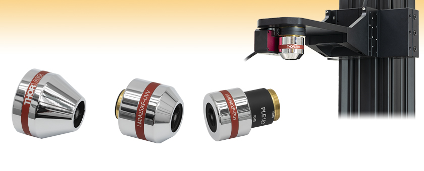
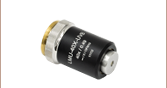
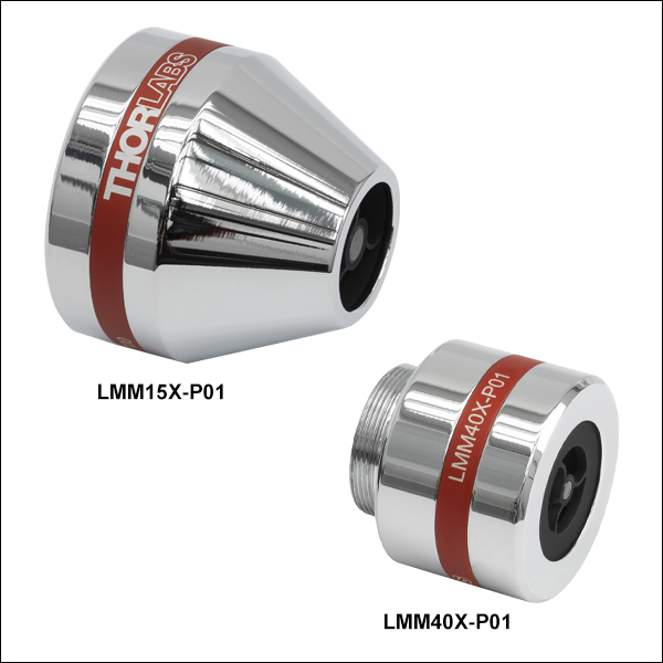
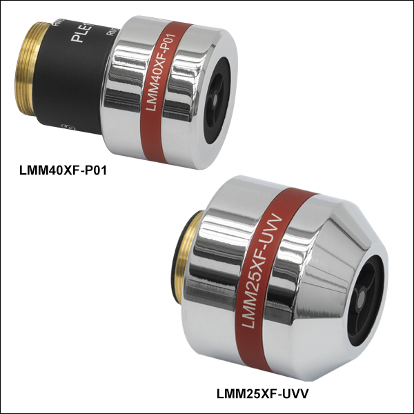
LMM15X-P01
450 nm - 20 µm,
Infinite Back Focal Length
LMM25XF-UVV
200 nm - 20 µm,
160 mm Back Focal Length
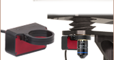
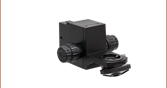
Application Idea
Reflective objective mounted in a
CSN100 Cerna® Nosepiece with a
PFM450E Piezo Objective Scanner.
Each Finite Conjugate 40X Objective
Includes a Parfocal Length Extender
(LMM40XF-P01 Shown)


Please Wait
| Objective Lens Selection Guide |
|---|
| Objectives |
| Super Apochromatic Microscope Objectives Microscopy Objectives, Dry Microscopy Objectives, Oil Immersion Physiology Objectives, Water Dipping or Immersion Phase Contrast Objectives Long Working Distance Objectives Reflective Microscopy Objectives UV Focusing Objectives VIS and NIR Focusing Objectives |
| Scan Lenses and Tube Lenses |
| Scan Lenses F-Theta Scan Lenses Infinity-Corrected Tube Lenses |
Applications
- Fourier Transform Infrared (FTIR) Spectroscopy
- Semiconductor Wafer Inspection
- Photolithography
- Ellipsometric Thin Film Measurements
- Hyperspectral Imaging
- Thermal Imaging Microscopy
- UV Fluorescence Imaging
- Laser Scanning
- White Light Imaging
- Materials Processing
- Ultrafast Laser Pulses
Click to Enlarge
Click Here for Raw Data
Figure 1.2 The reflectance plot shows the reflectance of the coated mirrors incorporated into our reflective microscope objectives. Please note that the data shown is per surface, i.e. for one reflection only. Light that enters the objective undergoes two reflections, which decreases the overall energy throughput from that shown here.
Click to Enlarge
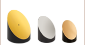
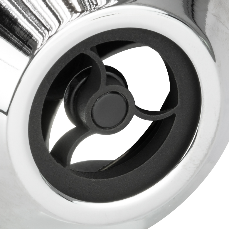
Figure 1.1 The front-mounted convex mirror being held by three 3-dimensional curved spider vanes.
Features
- 15X, 25X, or 40X Magnification (0.3 NA, 0.4 NA, or 0.5 NA, Respectively)
- Infinity-Corrected or 160 mm Back Focal Length
- Schwarzschild Design and Diffraction-Limited Performance
- All-Reflective Optical Design Introduces No Chromatic Aberration
- Two Broadband Reflective Coatings Available (See Plots in Figure 1.2)
- UV-Enhanced Aluminum: Rabs > 80% for 200 nm - 20 µm
- Protected Silver: Ravg > 97% for 450 nm - 2 µm;
Ravg > 95% for 2 µm - 20 µm - RMS (0.800"-36) Threads for Compatibility with Most Microscopes
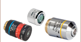
Thorlabs' Reflective Microscope Objectives consist of reflective surfaces that focus light without introducing chromatic aberration. We offer objectives with two broadband reflective coatings, three magnifications, and in either infinity-corrected or finite conjugate versions. Based on the classical Schwarzschild design, these objectives are corrected for third-order spherical aberration, coma, and astigmatism, and have negligible higher-order aberrations, resulting in diffraction-limited performance. Please refer to the Wavefront Error tab for more details. These advantages make reflective objectives well suited for applications that require longer working distances than those provided by typical refractive objectives.
These objectives are available with one of two reflective coatings: a UV-enhanced aluminum coating for >80% absolute reflectance in the 200 nm - 20 µm wavelength range or a protected silver coating for >97% average reflectance in the 450 nm - 2 µm wavelength range and >95% average reflectance in the 2 µm - 20 µm wavelength range. Note that this reflectance is for a single coated surface and incoming light is reflected by two coated surfaces. Refer to the tables below for additional specifications.
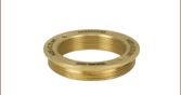
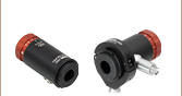
These objectives are RMS threaded (0.800"-36) for compatibility with most manufacturers' microscopes. As shown in the images at the top of the page, the housings are engraved with the part number for easy identification. Additionally, Thorlabs also offers the M32RMSS brass thread adapter to convert RMS threads to M32 x 0.75 threads.
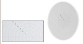
Each reflective objective incorporates a small convex secondary mirror that is mounted on three 3-dimensional curved spider vanes. Also referred to as legs, these are visible at the tip of the objective in Figures 1.1 and 1.4. Please note that this mirror and the spider vanes act as a central obscuration (blocked area; refer to Figure 1.5) that causes a reduction of the contrast for low to mid spatial frequencies. The spider vanes also cause a faint diffraction pattern. Compared to straight spider vanes, the 3-dimensional curved spider vanes minimize the diffraction patterns and keep the obscuration ratio at a minimum. Please refer to the Obscuration tab for more information. Alternatively, our Zemax files can provide more details on the effect of the obscuration.
The 15X and 25X objectives have a special tapered mechanical design, which maximize the space for an access to the sample from the side of the objectives. Please see our mechanical drawing for detailed dimensions.
For custom objectives intended for vacuum or low-temperature applications, as well as non-magnetic versions of our reflective objectives, please contact Tech Support.
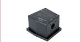
Cleaning and Storage
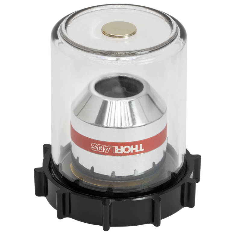
To clean these objectives, we recommend using an inert gas, such as nitrogen or argon, to blow away contaminants. Solvents and liquids should not be used. If inert gas is not sufficient, please contact Tech Support to inquire about returning the optic to Thorlabs for cleaning/testing. All objectives are shipped inside a protective container, as shown in the photo below. When not in use, we recommend using the included clear case to protect the objective. For replacement or substitution, an objective case (OC2RMS lid and OC22 canister) and aluminum cap (RMSCP1) are also available for purchase separately.
Click to Enlarge
Figure 1.3 All objectives are shipped inside a storage case composed of an OC22 Canister and OC2RMS Lid.
Click to Enlarge
Figure 1.4 View of curved spider vanes from the backside of the objective, showing the equal thickness of
the vanes.
Click to Enlarge
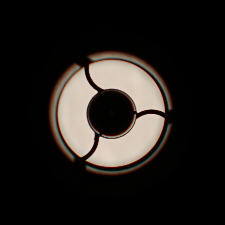
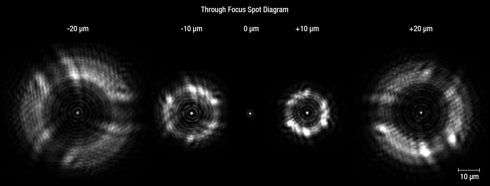
Figure 1.5 These images were taken with a reflective objective with curved spider vanes at various offsets from the focal plane. When the spot is accurately focused (0 µm offset in the diagram above), the obscuration effect disappears within the central Airy disc and cannot be resolved any longer.
Click to Enlarge
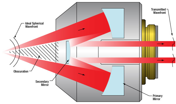
Figure 2.1 The wavefront is partially obscured by the secondary mirror and spider vanes before being reflected by the primary mirror and then the
secondary mirror.
Diffraction-Limited and Minimal Spherical Aberration, Coma, and Astigmatism
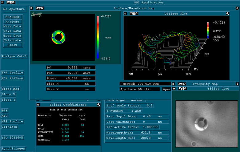
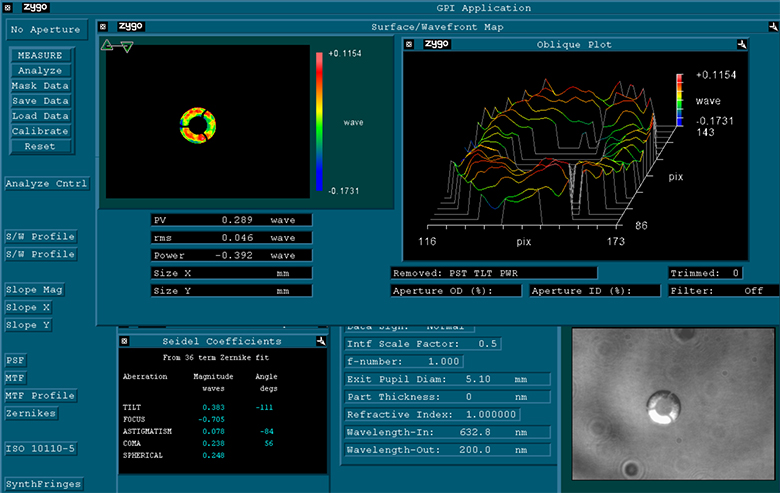
The interferograms were determined with a 633 nm laser source. However, the peak-to-valley (P-V) and RMS wavefront error results are normalized to the output wavelength of 200 nm by a setting in the software. They measure the transmitted wavefront error of reflective objectives to quantitatively show the diffraction-limited design of these objectives. The extracted values in Tables 2.5, 2.6, and 2.7 represent the performance of typical objectives. The interferograms also show these objectives correct 3rd order Seidel aberrations, such as astigmatism and coma.
The intensity maps at the bottom right of Figures 2.2, 2.3, and 2.4 also show the obscured area in the center of the imaging system. The obscurations are caused by the convex mirror and the spider vane assembly holding the convex mirror in place.
Please note that the wavefront and aberration performance of these objectives is consistent regardless of the type of reflective coating, and thus the images and data below apply to the protected silver-coated (-P01) objectives as well as the UV-enhanced-aluminum-coated objectives (-UVV). The type of mirror coating primarily affects the light throughput at a given wavelength.
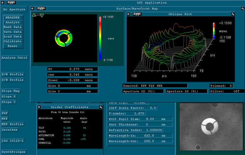
| Table 2.5 Sample LMM15X-UVV Performancea | ||
|---|---|---|
| Transmitted Wavefront Error | 0.040λ (RMS) 0.279λ (P-V) |
|
| Table 2.6 Sample LMM25X-UVV Performancea | ||
|---|---|---|
| Transmitted Wavefront Error | 0.034λ (RMS) 0.213λ (P-V) |
|
| Table 2.7 Sample LMM40X-UVV Performancea | ||
|---|---|---|
| Transmitted Wavefront Error | 0.046λ (RMS) 0.289λ (P-V) |
|
Click to Enlarge
Figure 3.1 The wavefront is partially obscured by the secondary mirror and spider vanes before being reflected by the primary mirror and then the secondary mirror.
Effects of Obscuration
Reflective objective designs incorporate a secondary mirror that is typically mounted on three spider vanes. The mirror and vanes create an obstruction to the entrance pupil (see Figures 3.1 and 3.2) that decreases transmitted light and modifies the diffraction pattern. Our Zemax files provide more detailed simulation data on the effects of the obscuration of our reflective objectives. Click on the red Document icon (![]() ) next to the item numbers below to access the Zemax file download. Our entire Zemax Catalog is also available.
) next to the item numbers below to access the Zemax file download. Our entire Zemax Catalog is also available.
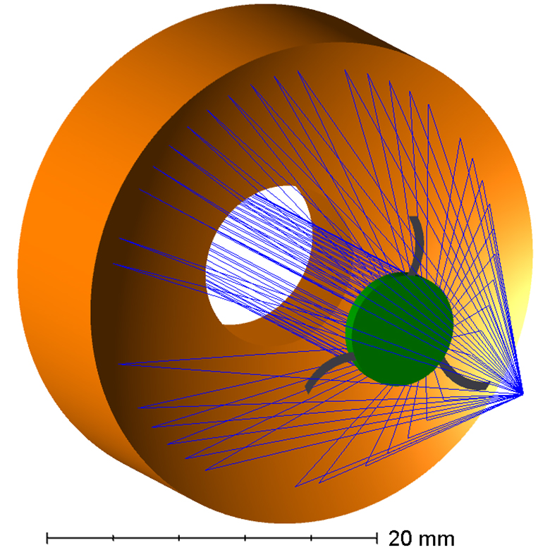
Central Obscuration
The central obscuration is caused by the convex secondary mirror (green mirrors in Figure 3.2) of the Schwarzschild objective. The value specified for the obscuration is the ratio of the obscured area to the entire area of the entrance pupil. If the entrance pupil is homogenously filled, the transmitted light would be reduced by the same factor as the area obscuration. Furthermore, the central obscuration in the entrance pupil results in a redistribution of the intensities of the diffraction rings. Compared to the point spread function of an unobscured system, the central obscuration causes a slightly smaller diameter of the central Airy disc, and thus a slightly higher resolution. However, the secondary maxima also increase in intensity as illustrated in Figure 3.3.
The redistribution of the diffraction intensities also affects the contrast of the image, which is evident in the Modulation Transfer Functions (MTF) shown in Figure 3.4. Compared to an unobscured optical system, the MTF for low and mid spatial frequencies will decrease as the central obscuration increases in size. Also, the MTF increases slightly at high spatial frequencies, which correlates with the slightly smaller central Airy disc (see Figure 3.3).
Click to Enlarge
Figure 3.2 This ray trace diagram illustrates the optics and obstructions in a reflective objective with three curved
spider vanes.
Click to Enlarge
Figure 3.3 This irradiance graph includes point spread functions and measured data of a gaussian beam through a reflective objective with 26% obscuration. The x-axis is the normalized distance from the theoretical maximum to the first minimum of the reflective objective.
Click to Enlarge
Figure 3.4 Obscurations impact the modulation transfer fuction (MTF) and image contrast. The theoretical MTF shown here is for a central circular obscuration with three spider vanes.
Spider Vane Obscuration
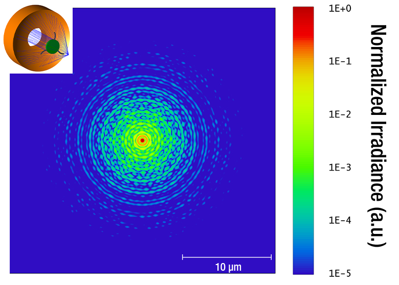
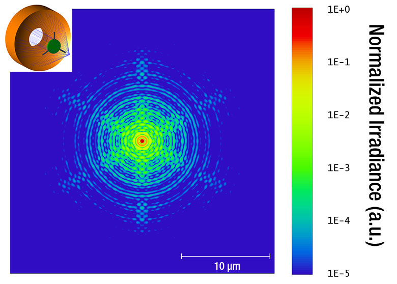
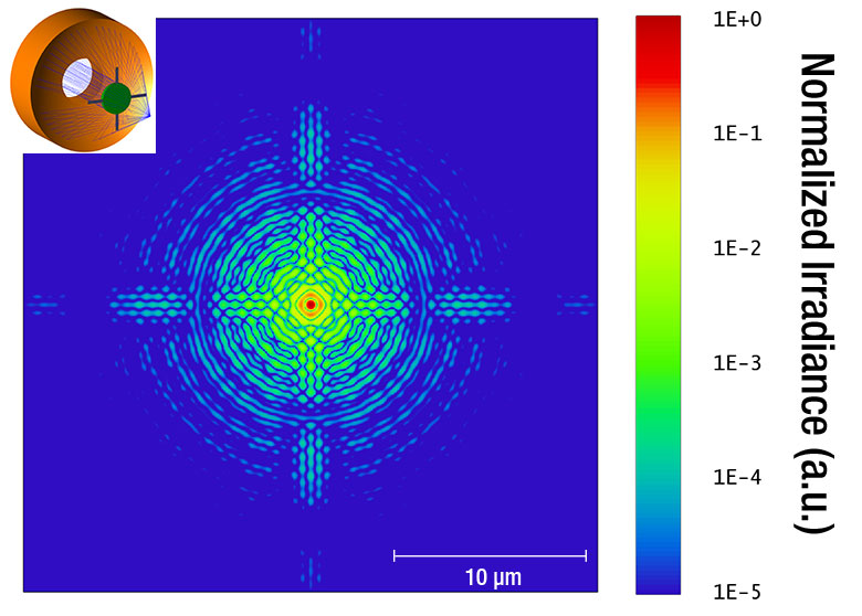
Besides the central obscuration, the amount and distribution of the diffracted energy is dependent on the width, shape, and number of spider vanes used to support the secondary mirror. The diffraction pattern in Figure 3.5 is produced by three curved spider vanes, like those illustrated in Figure 3.2. The objectives sold on this page incorporate three curved vanes. Please observe that the plots are given with a logarithmical intensity scale over five orders of magnitude for a better visualization of the diffraction effects. Figure 3.6 illustrates a diffraction pattern produced by three straight spider vanes. It can be seen that the amount of the diffracted energy will almost be the same, however, with a more uneven distribution. For comparison purposes, Figure 3.7 presents the pattern resulting from the use of four straight vanes.
Click to Enlarge
Figure 3.5 Diffraction Effect from Three Curved Spider Vanes
Click to Enlarge
Figure 3.6 Diffraction Effect from Three Straight Spider Vanes
Click to Enlarge
Figure 3.7 Diffraction Effect from Four Straight Spider Vanes
| Table 89A Chromatic Aberration Correction per ISO Standard 19012-2 | ||
|---|---|---|
| Objective Class | Common Abbreviations | Axial Focal Shift Tolerancesa |
| Achromat | ACH, ACHRO, ACHROMAT | |δC' - δF'| ≤ 2 x δob |
| Semiapochromat (or Fluorite) |
SEMIAPO, FL, FLU | |δC' - δF'| ≤ 2 x δob |δF' - δe| ≤ 2.5 x δob |δC' - δe| ≤ 2.5 x δob |
| Apochromat | APO | |δC' - δF'| ≤ 2 x δob |δF' - δe| ≤ δob |δC' - δe| ≤ δob |
| Super Apochromat | SAPO | See Footnote b |
| Improved Visible Apochromat | VIS+ | See Footnotes b and c |
Parts of a Microscope Objective
Click on each label for more details.
Figure 89C This microscope objective serves only as an example. The features noted above with an asterisk may not be present on all objectives; they may be added, relocated, or removed from objectives based on the part's needs and intended application space.
Objective Tutorial
This tutorial describes features and markings of objectives and what they tell users about an objective's performance.
Objective Class and Aberration Correction
Objectives are commonly divided by their class. An objective's class creates a shorthand for users to know how the objective is corrected for imaging aberrations. There are two types of aberration corrections that are specified by objective class: field curvature and chromatic aberration.
Field curvature (or Petzval curvature) describes the case where an objective's plane of focus is a curved spherical surface. This aberration makes widefield imaging or laser scanning difficult, as the corners of an image will fall out of focus when focusing on the center. If an objective's class begins with "Plan", it will be corrected to have a flat plane of focus.
Images can also exhibit chromatic aberrations, where colors originating from one point are not focused to a single point. To strike a balance between an objective's performance and the complexity of its design, some objectives are corrected for these aberrations at a finite number of target wavelengths.
Five objective classes are shown in Table 89A; only three common objective classes are defined under the International Organization for Standards ISO 19012-2: Microscopes -- Designation of Microscope Objectives -- Chromatic Correction. Due to the need for better performance, we have added two additional classes that are not defined in the ISO classes.
Immersion Methods
Click on each image for more details.
Figure 89B Objectives can be divided by what medium they are designed to image through. Dry objectives are used in air; whereas dipping and immersion objectives are designed to operate with a fluid between the objective and the front element of the sample.
| Glossary of Terms | |
|---|---|
| Back Focal Length and Infinity Correction | The back focal length defines the location of the intermediate image plane. Most modern objectives will have this plane at infinity, known as infinity correction, and will signify this with an infinity symbol (∞). Infinity-corrected objectives are designed to be used with a tube lens between the objective and eyepiece. Along with increasing intercompatibility between microscope systems, having this infinity-corrected space between the objective and tube lens allows for additional modules (like beamsplitters, filters, or parfocal length extenders) to be placed in the beam path. Note that older objectives and some specialty objectives may have been designed with finite back focal lengths. In their inception, finite back focal length objectives were meant to interface directly with the objective's eyepiece. |
| Entrance Pupil Diameter (EP) | The entrance pupil diameter (EP), sometimes referred to as the entrance aperture diameter, corresponds to the appropriate beam diameter one should use to allow the objective to function properly. EP = 2 × NA × Effective Focal Length |
| Field Number (FN) and Field of View (FOV) |
The field number corresponds to the diameter of the field of view in object space (in millimeters) multiplied by the objective's magnification. Field Number = Field of View Diameter × Magnification |
| Magnification (M) | The magnification (M) of an objective is the lens tube focal length (L) divided by the objective's effective focal length (F). Effective focal length is sometimes abbreviated EFL: M = L / EFL . The total magnification of the system is the magnification of the objective multiplied by the magnification of the eyepiece or camera tube. The specified magnification on the microscope objective housing is accurate as long as the objective is used with a compatible tube lens focal length. Objectives will have a colored ring around their body to signify their magnification. This is fairly consistent across manufacturers; see the Parts of a Microscope Objective section for more details. |
| Numerical Aperture (NA) | Numerical aperture, a measure of the acceptance angle of an objective, is a dimensionless quantity. It is commonly expressed as: NA = ni × sinθa where θa is the maximum 1/2 acceptance angle of the objective, and ni is the index of refraction of the immersion medium. This medium is typically air, but may also be water, oil, or other substances. |
| Working Distance (WD) |
The working distance, often abbreviated WD, is the distance between the front element of the objective and the top of the specimen (in the case of objectives that are intended to be used without a cover glass) or top of the cover glass, depending on the design of the objective. The cover glass thickness specification engraved on the objective designates whether a cover glass should be used. |
A cover glass, or coverslip, is a small, thin sheet of glass that can be placed on a wet sample to create a flat surface to image across.
The most common, a standard #1.5 cover glass, is designed to be 0.17 mm thick. Due to variance in the manufacturing process the actual thickness may be different. The correction collar present on select objectives is used to compensate for cover glasses of different thickness by adjusting the relative position of internal optical elements. Note that many objectives do not have a variable cover glass correction, in which case the objectives have no correction collar. For example, an objective could be designed for use with only a #1.5 cover glass. This collar may also be located near the bottom of the objective, instead of the top as shown in the diagram.
Click to Enlarge
The graph above shows the magnitude of spherical aberration versus the thickness of the coverslip used for 632.8 nm light. For the typical coverslip thickness of 0.17 mm, the spherical aberration caused by the coverslip does not exceed the diffraction-limited aberration for objectives with NA up to 0.40.
When viewing an image with a camera, the system magnification is the product of the objective and camera tube magnifications. When viewing an image with trinoculars, the system magnification is the product of the objective and eyepiece magnifications.

| Manufacturer | Tube Lens Focal Length |
|---|---|
| Leica | f = 200 mm |
| Mitutoyo | f = 200 mm |
| Nikon | f = 200 mm |
| Olympus | f = 180 mm |
| Thorlabs | f = 200 mm |
| Zeiss | f = 165 mm |
Magnification and Sample Area Calculations
Magnification
The magnification of a system is the multiplicative product of the magnification of each optical element in the system. Optical elements that produce magnification include objectives, camera tubes, and trinocular eyepieces, as shown in the drawing to the right. It is important to note that the magnification quoted in these products' specifications is usually only valid when all optical elements are made by the same manufacturer. If this is not the case, then the magnification of the system can still be calculated, but an effective objective magnification should be calculated first, as described below.
To adapt the examples shown here to your own microscope, please use our Magnification and FOV Calculator, which is available for download by clicking on the red button above. Note the calculator is an Excel spreadsheet that uses macros. In order to use the calculator, macros must be enabled. To enable macros, click the "Enable Content" button in the yellow message bar upon opening the file.
Example 1: Camera Magnification
When imaging a sample with a camera, the image is magnified by the objective and the camera tube. If using a 20X Nikon objective and a 0.75X Nikon camera tube, then the image at the camera has 20X × 0.75X = 15X magnification.
Example 2: Trinocular Magnification
When imaging a sample through trinoculars, the image is magnified by the objective and the eyepieces in the trinoculars. If using a 20X Nikon objective and Nikon trinoculars with 10X eyepieces, then the image at the eyepieces has 20X × 10X = 200X magnification. Note that the image at the eyepieces does not pass through the camera tube, as shown by the drawing to the right.
Using an Objective with a Microscope from a Different Manufacturer
Magnification is not a fundamental value: it is a derived value, calculated by assuming a specific tube lens focal length. Each microscope manufacturer has adopted a different focal length for their tube lens, as shown by the table to the right. Hence, when combining optical elements from different manufacturers, it is necessary to calculate an effective magnification for the objective, which is then used to calculate the magnification of the system.
The effective magnification of an objective is given by Equation 1:
 |
(Eq. 1) |
Here, the Design Magnification is the magnification printed on the objective, fTube Lens in Microscope is the focal length of the tube lens in the microscope you are using, and fDesign Tube Lens of Objective is the tube lens focal length that the objective manufacturer used to calculate the Design Magnification. These focal lengths are given by the table to the right.
Note that Leica, Mitutoyo, Nikon, and Thorlabs use the same tube lens focal length; if combining elements from any of these manufacturers, no conversion is needed. Once the effective objective magnification is calculated, the magnification of the system can be calculated as before.
Example 3: Trinocular Magnification (Different Manufacturers)
When imaging a sample through trinoculars, the image is magnified by the objective and the eyepieces in the trinoculars. This example will use a 20X Olympus objective and Nikon trinoculars with 10X eyepieces.
Following Equation 1 and the table to the right, we calculate the effective magnification of an Olympus objective in a Nikon microscope:
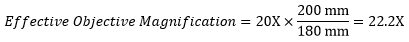 |
The effective magnification of the Olympus objective is 22.2X and the trinoculars have 10X eyepieces, so the image at the eyepieces has 22.2X × 10X = 222X magnification.
Sample Area When Imaged on a Camera
When imaging a sample with a camera, the dimensions of the sample area are determined by the dimensions of the camera sensor and the system magnification, as shown by Equation 2.
 |
(Eq. 2) |
The camera sensor dimensions can be obtained from the manufacturer, while the system magnification is the multiplicative product of the objective magnification and the camera tube magnification (see Example 1). If needed, the objective magnification can be adjusted as shown in Example 3.
As the magnification increases, the resolution improves, but the field of view also decreases. The dependence of the field of view on magnification is shown in the schematic to the right.
Example 4: Sample Area
The dimensions of the camera sensor in Thorlabs' previous-generation 1501M-USB Scientific Camera are 8.98 mm × 6.71 mm. If this camera is used with the Nikon objective and trinoculars from Example 1, which have a system magnification of 15X, then the image area is:
 |
Sample Area Examples
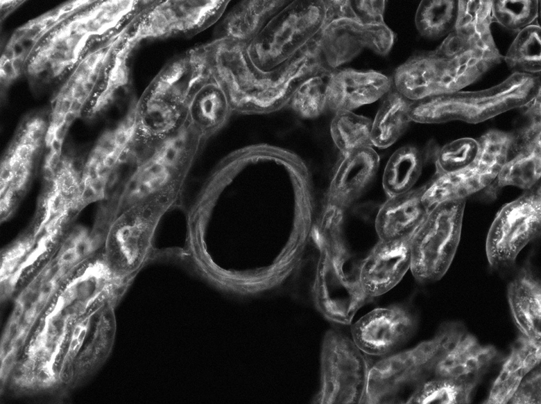
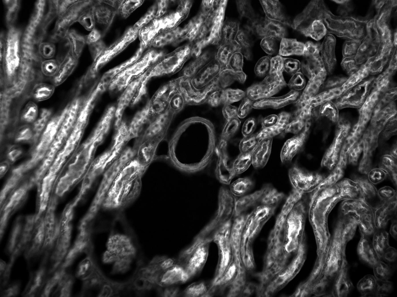
The images of a mouse kidney below were all acquired using the same objective and the same camera. However, the camera tubes used were different. Read from left to right, they demonstrate that decreasing the camera tube magnification enlarges the field of view at the expense of the size of the details in the image.

Resolution Tutorial
An important parameter in many imaging applications is the resolution of the objective. This tutorial describes the different conventions used to define an objective's resolution. Thorlabs provides the theoretical Rayleigh resolution for all of the imaging objectives offered on our site; the other conventions are presented for informational purposes.
Resolution
The resolution of an objective refers to its ability to distinguish closely-spaced features of an object. This is often theoretically quantified by considering an object that consists of two point sources and asking at what minimum separation can these two point sources be resolved. When a point source is imaged, rather than appearing as a singular bright point, it will appear as a broadened intensity profile due to the effects of diffraction. This profile, known as an Airy disk, consists of an intense central peak with surrounding rings of much lesser intensity. The image produced by two point sources in proximity to one another will therefore consist of two overlapping Airy disk profiles, and the resolution of the objective is therefore determined by the minimum spacing at which the two profiles can be uniquely identified. There is no fundamental criterion for establishing what exactly it means for the two profiles to be resolved and, as such, there are a few criteria that are observed in practice. In microscopic imaging applications, the two most commonly used criteria are the Rayleigh and Abbe criteria. A third criterion, more common in astronomical applications, is the Sparrow criterion.
Rayleigh Criterion
The Rayleigh criterion states that two overlapping Airy disk profiles are resolved when the first intensity minimum of one profile coincides with the intensity maximum of the other profile [1]. It can be shown that the first intensity minimum occurs at a radius of 1.22λf/D from the central maximum, where λ is the wavelength of the light, f is the focal length of the objective, and D is the entrance pupil diameter. Thus, in terms of the numerical aperture (NA = 0.5*D/f), the Rayleigh resolution is:
rR = 0.61λ/NA
An idealized image of two Airy disks separated by a distance equal to the Rayleigh resolution is shown in the figure to the left below; the illumination source has been assumed to be incoherent. A corresponding horizontal line cut across the intensity maxima is plotted to the right. The vertical dashed lines in the intensity profile show that the maximum of each individual Airy disk overlaps with the neighboring minimum. Between the two maxima, there is a local minimum which appears in the image as a gray region between the two white peaks.
 Click to Enlarge
Left: Two point sources are considered resolved when separated by the Rayleigh resolution. The gray region between the two white peaks is clearly visible.
Above: The vertical dashed lines show how the maximum of each intensity profile overlaps with the first minimum of the other.

Thorlabs provides the theoretical Rayleigh resolution for all of the imaging objectives offered on our site in their individual product presentations.
Abbe Criterion
The Abbe theory describes image formation as a double process of diffraction [2]. Within this framework, if two features separated by a distance d are to be resolved, at a minimum both the zeroth and first orders of diffraction must be able to pass through the objective's aperture. Since the first order of diffraction appears at the angle: sin(θ1) = λ/d, the minimum object separation, or equivalently the resolution of the objective, is given by d = λ/n*sin(α), where α is the angular semi-aperture of the objective and a factor of n has been inserted to account for the refractive index of the imaging medium. This result overestimates the actual limit by a factor of 2 because both first orders of diffraction are assumed to be accepted by the objective, when in fact only one of the first orders must pass through along with the zeroth order. Dividing the above result by a factor of 2 and using the definition of the numerical aperture (NA = n*sin(α)) gives the famous Abbe resolution limit:
rA = 0.5λ/NA
In the image below, two Airy disks are shown separated by the Abbe resolution limit. Compared to the Rayleigh limit, the decrease in intensity at the origin is much harder to discern. The horizontal line cut to the right shows that the intensity decreases by only ≈2%.
 Click to Enlarge
Left: Two point sources separated by the Abbe resolution limit. Though observable, the contrast between the maxima and central minimum is much weaker compared to the Rayleigh limit.
Above: The line cut shows the small intensity dip between the two maxima.

Sparrow Criterion
For point source separations corresponding to the Rayleigh and Abbe resolution criteria, the combined intensity profile has a local minimum located at the origin between the two maxima. In a sense, this feature is what allows the two point sources to be resolved. That is to say, if the sources' separation is further decreased beyond the Abbe resolution limit, the two individual maxima will merge into one central maximum and resolving the two individual contributions will no longer be possible. The Sparrow criterion posits that the resolution limit is reached when the crossover from a central minimum to a central maximum occurs.
At the Sparrow resolution limit, the center of the combined intensity profile is flat, which implies that the derivative with respect to position is zero at the origin. However, this first derivative at the origin is always zero, given that it is either a local minimum or maximum of the combined intensity profile (strictly speaking, this is only the case if the sources have equal intensities). Consider then, that because the Sparrow resolution limit occurs when the origin's intensity changes from a local minimum to a maximum, that the second derivative must be changing sign from positive to negative. The Sparrow criterion is thus a condition that is imposed upon the second derivative, namely that the resolution limit occurs when the second derivative is zero [3]. Applying this condition to the combined intensity profile of two Airy disks leads to the Sparrow resolution:
rS = 0.47λ/NA
The image to the left below shows two Airy disks separated by the Sparrow resolution limit. As described above, the intensity is constant in the region between the two peaks and there is no intensity dip at the origin. In the line cut to the right, the constant intensity near the origin is confirmed.
 Click to Enlarge
Left: Two Airy disk profiles separated by the Sparrow resolution limit. Note that, unlike the Rayleigh or Abbe limits, there is no decrease in intensity at the origin.
Above: At the Sparrow resolution limit, the combined intensity is a constant near the origin. The scale here has been normalized to 1.

References
[1] Eugene Hecht, "Optics," 4th Ed., Addison-Wesley (2002)
[2] S.G. Lipson, H. Lipson, and D.S. Tannhauser, "Optical Physics," 3rd Ed., Cambridge University Press (1995)
[3] C.M. Sparrow, "On Spectroscopic Resolving Power," Astrophys. J. 44, 76-87 (1916)
| Table 7.1 Damage Threshold Specifications | ||
|---|---|---|
| Coating Type | Laser Type | Damage Threshold |
| UV-Enhanced Aluminum (-UVV) |
Pulsed | 0.3 J/cm2 (355 nm, 10 ns, 10 Hz, Ø0.381 mm) |
| Protected Silver (-P01) | Pulsed | 1.0 J/cm2 (1064 nm, 10 ns, 10 Hz, Ø0.230 mm) |
Damage Threshold Data for Thorlabs' Reflective Objectives
The specifications in Table 7.1 are measured data for the mirrors used in Thorlabs' reflective microscope objectives. Damage threshold specifications are constant for all objectives with a given coating type, regardless of magnification or other specs.
Laser Induced Damage Threshold Tutorial
The following is a general overview of how laser induced damage thresholds are measured and how the values may be utilized in determining the appropriateness of an optic for a given application. When choosing optics, it is important to understand the Laser Induced Damage Threshold (LIDT) of the optics being used. The LIDT for an optic greatly depends on the type of laser you are using. Continuous wave (CW) lasers typically cause damage from thermal effects (absorption either in the coating or in the substrate). Pulsed lasers, on the other hand, often strip electrons from the lattice structure of an optic before causing thermal damage. Note that the guideline presented here assumes room temperature operation and optics in new condition (i.e., within scratch-dig spec, surface free of contamination, etc.). Because dust or other particles on the surface of an optic can cause damage at lower thresholds, we recommend keeping surfaces clean and free of debris. For more information on cleaning optics, please see our Optics Cleaning tutorial.
Testing Method
Thorlabs' LIDT testing is done in compliance with ISO/DIS 11254 and ISO 21254 specifications.
First, a low-power/energy beam is directed to the optic under test. The optic is exposed in 10 locations to this laser beam for 30 seconds (CW) or for a number of pulses (pulse repetition frequency specified). After exposure, the optic is examined by a microscope (~100X magnification) for any visible damage. The number of locations that are damaged at a particular power/energy level is recorded. Next, the power/energy is either increased or decreased and the optic is exposed at 10 new locations. This process is repeated until damage is observed. The damage threshold is then assigned to be the highest power/energy that the optic can withstand without causing damage. A histogram such as that below represents the testing of one BB1-E02 mirror.
The photograph above is a protected aluminum-coated mirror after LIDT testing. In this particular test, it handled 0.43 J/cm2 (1064 nm, 10 ns pulse, 10 Hz, Ø1.000 mm) before damage.
| Example Test Data | |||
|---|---|---|---|
| Fluence | # of Tested Locations | Locations with Damage | Locations Without Damage |
| 1.50 J/cm2 | 10 | 0 | 10 |
| 1.75 J/cm2 | 10 | 0 | 10 |
| 2.00 J/cm2 | 10 | 0 | 10 |
| 2.25 J/cm2 | 10 | 1 | 9 |
| 3.00 J/cm2 | 10 | 1 | 9 |
| 5.00 J/cm2 | 10 | 9 | 1 |
According to the test, the damage threshold of the mirror was 2.00 J/cm2 (532 nm, 10 ns pulse, 10 Hz, Ø0.803 mm). Please keep in mind that these tests are performed on clean optics, as dirt and contamination can significantly lower the damage threshold of a component. While the test results are only representative of one coating run, Thorlabs specifies damage threshold values that account for coating variances.
Continuous Wave and Long-Pulse Lasers
When an optic is damaged by a continuous wave (CW) laser, it is usually due to the melting of the surface as a result of absorbing the laser's energy or damage to the optical coating (antireflection) [1]. Pulsed lasers with pulse lengths longer than 1 µs can be treated as CW lasers for LIDT discussions.
When pulse lengths are between 1 ns and 1 µs, laser-induced damage can occur either because of absorption or a dielectric breakdown (therefore, a user must check both CW and pulsed LIDT). Absorption is either due to an intrinsic property of the optic or due to surface irregularities; thus LIDT values are only valid for optics meeting or exceeding the surface quality specifications given by a manufacturer. While many optics can handle high power CW lasers, cemented (e.g., achromatic doublets) or highly absorptive (e.g., ND filters) optics tend to have lower CW damage thresholds. These lower thresholds are due to absorption or scattering in the cement or metal coating.

LIDT in linear power density vs. pulse length and spot size. For long pulses to CW, linear power density becomes a constant with spot size. This graph was obtained from [1].
Pulsed lasers with high pulse repetition frequencies (PRF) may behave similarly to CW beams. Unfortunately, this is highly dependent on factors such as absorption and thermal diffusivity, so there is no reliable method for determining when a high PRF laser will damage an optic due to thermal effects. For beams with a high PRF both the average and peak powers must be compared to the equivalent CW power. Additionally, for highly transparent materials, there is little to no drop in the LIDT with increasing PRF.
In order to use the specified CW damage threshold of an optic, it is necessary to know the following:
- Wavelength of your laser
- Beam diameter of your beam (1/e2)
- Approximate intensity profile of your beam (e.g., Gaussian)
- Linear power density of your beam (total power divided by 1/e2 beam diameter)
Thorlabs expresses LIDT for CW lasers as a linear power density measured in W/cm. In this regime, the LIDT given as a linear power density can be applied to any beam diameter; one does not need to compute an adjusted LIDT to adjust for changes in spot size, as demonstrated by the graph to the right. Average linear power density can be calculated using the equation below.
The calculation above assumes a uniform beam intensity profile. You must now consider hotspots in the beam or other non-uniform intensity profiles and roughly calculate a maximum power density. For reference, a Gaussian beam typically has a maximum power density that is twice that of the uniform beam (see lower right).
Now compare the maximum power density to that which is specified as the LIDT for the optic. If the optic was tested at a wavelength other than your operating wavelength, the damage threshold must be scaled appropriately. A good rule of thumb is that the damage threshold has a linear relationship with wavelength such that as you move to shorter wavelengths, the damage threshold decreases (i.e., a LIDT of 10 W/cm at 1310 nm scales to 5 W/cm at 655 nm):
While this rule of thumb provides a general trend, it is not a quantitative analysis of LIDT vs wavelength. In CW applications, for instance, damage scales more strongly with absorption in the coating and substrate, which does not necessarily scale well with wavelength. While the above procedure provides a good rule of thumb for LIDT values, please contact Tech Support if your wavelength is different from the specified LIDT wavelength. If your power density is less than the adjusted LIDT of the optic, then the optic should work for your application.
Please note that we have a buffer built in between the specified damage thresholds online and the tests which we have done, which accommodates variation between batches. Upon request, we can provide individual test information and a testing certificate. The damage analysis will be carried out on a similar optic (customer's optic will not be damaged). Testing may result in additional costs or lead times. Contact Tech Support for more information.
Pulsed Lasers
As previously stated, pulsed lasers typically induce a different type of damage to the optic than CW lasers. Pulsed lasers often do not heat the optic enough to damage it; instead, pulsed lasers produce strong electric fields capable of inducing dielectric breakdown in the material. Unfortunately, it can be very difficult to compare the LIDT specification of an optic to your laser. There are multiple regimes in which a pulsed laser can damage an optic and this is based on the laser's pulse length. The highlighted columns in the table below outline the relevant pulse lengths for our specified LIDT values.
Pulses shorter than 10-9 s cannot be compared to our specified LIDT values with much reliability. In this ultra-short-pulse regime various mechanics, such as multiphoton-avalanche ionization, take over as the predominate damage mechanism [2]. In contrast, pulses between 10-7 s and 10-4 s may cause damage to an optic either because of dielectric breakdown or thermal effects. This means that both CW and pulsed damage thresholds must be compared to the laser beam to determine whether the optic is suitable for your application.
| Pulse Duration | t < 10-9 s | 10-9 < t < 10-7 s | 10-7 < t < 10-4 s | t > 10-4 s |
|---|---|---|---|---|
| Damage Mechanism | Avalanche Ionization | Dielectric Breakdown | Dielectric Breakdown or Thermal | Thermal |
| Relevant Damage Specification | No Comparison (See Above) | Pulsed | Pulsed and CW | CW |
When comparing an LIDT specified for a pulsed laser to your laser, it is essential to know the following:
LIDT in energy density vs. pulse length and spot size. For short pulses, energy density becomes a constant with spot size. This graph was obtained from [1].
- Wavelength of your laser
- Energy density of your beam (total energy divided by 1/e2 area)
- Pulse length of your laser
- Pulse repetition frequency (prf) of your laser
- Beam diameter of your laser (1/e2 )
- Approximate intensity profile of your beam (e.g., Gaussian)
The energy density of your beam should be calculated in terms of J/cm2. The graph to the right shows why expressing the LIDT as an energy density provides the best metric for short pulse sources. In this regime, the LIDT given as an energy density can be applied to any beam diameter; one does not need to compute an adjusted LIDT to adjust for changes in spot size. This calculation assumes a uniform beam intensity profile. You must now adjust this energy density to account for hotspots or other nonuniform intensity profiles and roughly calculate a maximum energy density. For reference a Gaussian beam typically has a maximum energy density that is twice that of the 1/e2 beam.
Now compare the maximum energy density to that which is specified as the LIDT for the optic. If the optic was tested at a wavelength other than your operating wavelength, the damage threshold must be scaled appropriately [3]. A good rule of thumb is that the damage threshold has an inverse square root relationship with wavelength such that as you move to shorter wavelengths, the damage threshold decreases (i.e., a LIDT of 1 J/cm2 at 1064 nm scales to 0.7 J/cm2 at 532 nm):
You now have a wavelength-adjusted energy density, which you will use in the following step.
Beam diameter is also important to know when comparing damage thresholds. While the LIDT, when expressed in units of J/cm², scales independently of spot size; large beam sizes are more likely to illuminate a larger number of defects which can lead to greater variances in the LIDT [4]. For data presented here, a <1 mm beam size was used to measure the LIDT. For beams sizes greater than 5 mm, the LIDT (J/cm2) will not scale independently of beam diameter due to the larger size beam exposing more defects.
The pulse length must now be compensated for. The longer the pulse duration, the more energy the optic can handle. For pulse widths between 1 - 100 ns, an approximation is as follows:
Use this formula to calculate the Adjusted LIDT for an optic based on your pulse length. If your maximum energy density is less than this adjusted LIDT maximum energy density, then the optic should be suitable for your application. Keep in mind that this calculation is only used for pulses between 10-9 s and 10-7 s. For pulses between 10-7 s and 10-4 s, the CW LIDT must also be checked before deeming the optic appropriate for your application.
Please note that we have a buffer built in between the specified damage thresholds online and the tests which we have done, which accommodates variation between batches. Upon request, we can provide individual test information and a testing certificate. Contact Tech Support for more information.
[1] R. M. Wood, Optics and Laser Tech. 29, 517 (1998).
[2] Roger M. Wood, Laser-Induced Damage of Optical Materials (Institute of Physics Publishing, Philadelphia, PA, 2003).
[3] C. W. Carr et al., Phys. Rev. Lett. 91, 127402 (2003).
[4] N. Bloembergen, Appl. Opt. 12, 661 (1973).

In order to illustrate the process of determining whether a given laser system will damage an optic, a number of example calculations of laser induced damage threshold are given below. For assistance with performing similar calculations, we provide a spreadsheet calculator that can be downloaded by clicking the LIDT Calculator button. To use the calculator, enter the specified LIDT value of the optic under consideration and the relevant parameters of your laser system in the green boxes. The spreadsheet will then calculate a linear power density for CW and pulsed systems, as well as an energy density value for pulsed systems. These values are used to calculate adjusted, scaled LIDT values for the optics based on accepted scaling laws. This calculator assumes a Gaussian beam profile, so a correction factor must be introduced for other beam shapes (uniform, etc.). The LIDT scaling laws are determined from empirical relationships; their accuracy is not guaranteed. Remember that absorption by optics or coatings can significantly reduce LIDT in some spectral regions. These LIDT values are not valid for ultrashort pulses less than one nanosecond in duration.
Figure 71A A Gaussian beam profile has about twice the maximum intensity of a uniform beam profile.
CW Laser Example
Suppose that a CW laser system at 1319 nm produces a 0.5 W Gaussian beam that has a 1/e2 diameter of 10 mm. A naive calculation of the average linear power density of this beam would yield a value of 0.5 W/cm, given by the total power divided by the beam diameter:
However, the maximum power density of a Gaussian beam is about twice the maximum power density of a uniform beam, as shown in Figure 71A. Therefore, a more accurate determination of the maximum linear power density of the system is 1 W/cm.
An AC127-030-C achromatic doublet lens has a specified CW LIDT of 350 W/cm, as tested at 1550 nm. CW damage threshold values typically scale directly with the wavelength of the laser source, so this yields an adjusted LIDT value:
The adjusted LIDT value of 350 W/cm x (1319 nm / 1550 nm) = 298 W/cm is significantly higher than the calculated maximum linear power density of the laser system, so it would be safe to use this doublet lens for this application.
Pulsed Nanosecond Laser Example: Scaling for Different Pulse Durations
Suppose that a pulsed Nd:YAG laser system is frequency tripled to produce a 10 Hz output, consisting of 2 ns output pulses at 355 nm, each with 1 J of energy, in a Gaussian beam with a 1.9 cm beam diameter (1/e2). The average energy density of each pulse is found by dividing the pulse energy by the beam area:
As described above, the maximum energy density of a Gaussian beam is about twice the average energy density. So, the maximum energy density of this beam is ~0.7 J/cm2.
The energy density of the beam can be compared to the LIDT values of 1 J/cm2 and 3.5 J/cm2 for a BB1-E01 broadband dielectric mirror and an NB1-K08 Nd:YAG laser line mirror, respectively. Both of these LIDT values, while measured at 355 nm, were determined with a 10 ns pulsed laser at 10 Hz. Therefore, an adjustment must be applied for the shorter pulse duration of the system under consideration. As described on the previous tab, LIDT values in the nanosecond pulse regime scale with the square root of the laser pulse duration:
This adjustment factor results in LIDT values of 0.45 J/cm2 for the BB1-E01 broadband mirror and 1.6 J/cm2 for the Nd:YAG laser line mirror, which are to be compared with the 0.7 J/cm2 maximum energy density of the beam. While the broadband mirror would likely be damaged by the laser, the more specialized laser line mirror is appropriate for use with this system.
Pulsed Nanosecond Laser Example: Scaling for Different Wavelengths
Suppose that a pulsed laser system emits 10 ns pulses at 2.5 Hz, each with 100 mJ of energy at 1064 nm in a 16 mm diameter beam (1/e2) that must be attenuated with a neutral density filter. For a Gaussian output, these specifications result in a maximum energy density of 0.1 J/cm2. The damage threshold of an NDUV10A Ø25 mm, OD 1.0, reflective neutral density filter is 0.05 J/cm2 for 10 ns pulses at 355 nm, while the damage threshold of the similar NE10A absorptive filter is 10 J/cm2 for 10 ns pulses at 532 nm. As described on the previous tab, the LIDT value of an optic scales with the square root of the wavelength in the nanosecond pulse regime:
This scaling gives adjusted LIDT values of 0.08 J/cm2 for the reflective filter and 14 J/cm2 for the absorptive filter. In this case, the absorptive filter is the best choice in order to avoid optical damage.
Pulsed Microsecond Laser Example
Consider a laser system that produces 1 µs pulses, each containing 150 µJ of energy at a repetition rate of 50 kHz, resulting in a relatively high duty cycle of 5%. This system falls somewhere between the regimes of CW and pulsed laser induced damage, and could potentially damage an optic by mechanisms associated with either regime. As a result, both CW and pulsed LIDT values must be compared to the properties of the laser system to ensure safe operation.
If this relatively long-pulse laser emits a Gaussian 12.7 mm diameter beam (1/e2) at 980 nm, then the resulting output has a linear power density of 5.9 W/cm and an energy density of 1.2 x 10⁻⁴ J/cm2 per pulse. This can be compared to the LIDT values for a WPQ10E-980 polymer zero-order quarter-wave plate, which are 5 W/cm for CW radiation at 810 nm and 5 J/cm2 for a 10 ns pulse at 810 nm. As before, the CW LIDT of the optic scales linearly with the laser wavelength, resulting in an adjusted CW value of 6 W/cm at 980 nm. On the other hand, the pulsed LIDT scales with the square root of the laser wavelength and the square root of the pulse duration, resulting in an adjusted value of 55 J/cm2 for a 1 µs pulse at 980 nm. The pulsed LIDT of the optic is significantly greater than the energy density of the laser pulse, so individual pulses will not damage the wave plate. However, the large average linear power density of the laser system may cause thermal damage to the optic, much like a high-power CW beam.
| Posted Comments: | |
Dovlet Seyit
(posted 2025-01-22 23:43:35.953) Hello, may I ask if you can provide custom options? We would like the spiders to curve in a reverse way so when two objectives are facing each other the spider obscurations match. srydberg
(posted 2025-01-28 04:15:28.0) Hello, thank you for your question! We have contacted you directly to discuss your application. user
(posted 2024-12-26 18:19:38.44) Hello,
I'm interested in using the reflective objective and white light to see the sample image (the sample has a structure with a size of 50 um x 50 um). Because the secondary mirror can block the entrance pupil, what does the sample image look like?
If you can provide some example images obtained by reflective objective, it would be helpful.
Thank you! srydberg
(posted 2025-01-07 07:47:49.0) Hello, thank you for contacting Thorlabs! We have emailed you a sample image taken with the LMM15X-P01. user
(posted 2024-07-04 12:21:42.14) Dear Madam or Sir,
I am interested in the cryocompatible version of this objective. Do you have a version that would be able to operate at 4K and also tolerate large magnetic fields? fnero
(posted 2024-07-09 02:20:33.0) Thank you for reaching out. We are able to offer some customizations, such as non-magnetic and vacuum compatible versions. We have reached out to you directly to discuss your application more in detail. Dovlet Seyit
(posted 2024-05-31 11:41:18.223) Any plans to make 100X finite? fnero
(posted 2024-08-21 05:00:21.0) Thank you for your feedback! We have contacted you directly to discuss your application. Dovlet Seyit
(posted 2024-02-21 09:20:54.553) May I ask which method used to measure PSF of these objective. I am curious because they match simulations pretty well,
Best,
Seyit. mkarlsson
(posted 2024-02-22 04:16:38.0) Hello, We've reached out to you directly to discuss this in more detail. Dovlet Seyit
(posted 2024-02-19 21:55:12.653) Hello,
For my application I will need EXACT MTF of my objective,
I can see that you measured and also simulated and they match perfectly,
May I ask if you provide analytical model of your simulations with the product so we can utilize?
Also may I ask which methods you used?
In short, I need exact MTF of my objective so I can exclude that from my system,
Best. mkarlsson
(posted 2024-02-21 08:28:00.0) Thank you for reaching out! The simulations are performed in Zemax. You can find Zemax-files under the red document icon next to the product number on the webpage. These can be used to simulate the point spread function and MTF for our reflective objectives. I've also reached out to you directly to discuss this further. Andreas Heinrich
(posted 2023-11-03 15:32:20.403) LMM40X-P01
I am interested in collecting light in a confocal setup at low temperatures (about 1 Kelvin) and in vacuum. Do you have experience with using these reflective objectives under those conditions?
I prefer a high NA for maximum light collection efficiency. A working distance of 5mm would be acceptable.
Can you advise? mkarlsson
(posted 2023-11-06 02:08:16.0) Thank you for your request! We have reached out to you directly to discuss your application further. user
(posted 2023-08-11 09:38:53.887) Hi, please contact me for a vacuum (and potentially cryogenically compatible) version of LMM40X-UVV. I'd also like to know the back focal plane location, and the fraction of the entrance pupil that is "active". Thanks! cdolbashian
(posted 2023-08-29 04:16:01.0) Thank you for reaching out to us with this inquiry! For future custom requests, please feel free to contact our Solutions team directly at Techsales@thorlabs.com. Regarding the back focal plane, this can be found in our zemax simulation file, but for those without a Zemax license, the back focal plane is located ~24.54mm past the first mechanical surface (approximately the same location as the spider vanes within the component). user
(posted 2022-04-12 14:39:10.563) Where is the back focal plane of these reflective objectives? jdelia
(posted 2022-04-20 10:21:27.0) Thank you for contacting Thorlabs. You unfortunately did not leave an email for us to contact you directly with this information. Please send an email to techsupport@thorlabs.com to request a diagram showing this. Ethel Chen
(posted 2021-03-20 22:06:35.997) Hello,
Are these objectives able to work at cryogenic temperature (~ 1K)? Are they able to work under strong magnetic field (~ 8T)?
Thanks in advance!
Ethel Chen YLohia
(posted 2021-03-23 11:13:18.0) Hello, we may be able to offer custom versions of these objectives for cryogenic applications. An applications engineer will reach to you directly to discuss this further. Greg Lafyatis
(posted 2020-04-15 12:12:32.377) specifically interested in this objective. YLohia
(posted 2020-04-15 02:36:27.0) Thank you for your interest in the LMM-40X-UVV-160. I have reached out to you directly to answer any questions you may have on this product. Greg Lafyatis
(posted 2020-04-15 12:10:24.993) Quick questions,
Are these UHV compatible?
What is there maximum temperature? (i.e. could they withstand a 150 C takeout?)
Thanks,
Greg Lafyatis YLohia
(posted 2020-04-22 09:04:28.0) Hello Greg, thank you for contacting Thorlabs. The 150 C temperature would be fine for our standard LMM-40x series objectives. Unfortunately, we do not have enough data to spec that this would be fine for 10^-10 torr vacuum levels. We do, however, use a minimal amount of adhesive in these objectives. Alternately, we could offer a custom objective that we would bond with vacuum compatible adhesives. Daniel Nikiforov
(posted 2019-08-22 01:03:59.95) Hello, I plan to use these objectives at cryogenic temperatures (down to T~2K). Are these objectives designed to be cooled (for moderate cooling rate ~20K/min)? Have these objectives been tested for repeatebile cooling to cruogenic temperatures? YLohia
(posted 2019-08-21 02:51:43.0) Hello, thank you for contacting Thorlabs. We may be able to offer a custom version of this item for such applications. I have reached out to you directly to discuss this further. user
(posted 2019-08-05 14:10:09.597) I am worried that the part of light incident on the center of the small secondary mirror and not coupled into the primary will get backreflected and cause problems in my setup. Does the objective design address this problem and how? If not, can you offer any option that does (e.g. making the center absorbing)? nreusch
(posted 2019-08-09 10:07:11.0) Thank you for the feedback! We can offer a special LMM, where we add an absorptive dot in the middle of the small mirror to reduce the back reflection. Please contact your local Tech Support team for a quotation. a.c.frangeskou
(posted 2017-02-02 06:18:19.603) Hi,
I'd like to clarify if the intensity profile you show on the wave-front error is the intensity profile at the focus of the objective. Does this mean it has a dark spot in the middle of the focus?
Thanks. tcampbell
(posted 2017-02-03 04:42:08.0) Thank you for your feedback! There will not be a dark spot in the center of the focus. We have updated the Overview and Obscuration tabs to provide additional details about the effects of the obscuration caused by the secondary mirror and spider vane supports. f.liu-2
(posted 2016-07-10 04:50:51.82) Hello, I plan to use this objective to focus a ns pulsed laser beam at 126 nm. Can you estimate the reflectance at this wavelength? Thanks. jlow
(posted 2016-07-12 08:06:37.0) Response from Jeremy at Thorlabs: The reflectance would be around 0% at 126nm. david.panak
(posted 2016-06-06 09:20:41.02) i would like to use this reflective objective to couple out of one of your MIR (na=0.26) fibers. Do you have a mounting system that could hold the fiber connector as well as the objective lens at the correct (adjustable) distance? besembeson
(posted 2016-06-08 09:12:08.0) Response from Bweh at Thorlabs USA: We have several mounting adapters (http://www.thorlabs.com/navigation.cfm?guide_ID=2327) and terminated fiber adapters (http://www.thorlabs.com/newgrouppage9.cfm?objectgroup_id=69&pn=SM1SMA) that can help achieve this. I will contact you to discuss a configuration suitable for your application. leo.basset
(posted 2016-05-25 18:05:40.663) Hi, I would like to know the total transmission of the objective in the range from about 450nm to the deepest wavelength observable with it. Is there a graph you could send me detailing these features?
If not I'd like to know it at least for a wavelength of 300nm.
Also I don't really understand what the Seidel coefficient really imply in terms of aberrations seen on the picture. I plan to use these for imaging applications, and I can't assess how much aberrations will distort my image, could you give me an estimation of this in simpler terms? besembeson
(posted 2016-05-27 01:46:46.0) Response from Bweh at Thorlabs USA: The total transmission of these objectives depend on several factors such as the beam size, intensity profile beside the mirror reflectivity. According to Zemax, the LMM-40X-UVV transmission in the 300-1500nm range is about 43%, assuming a 5mm diameter Gaussian input and ideal 100% mirrors. At 355nm, with about 85% mirror reflectivity, total transmission will be about 31%.
The Seidel coefficients correspond to third order monochromatic aberrations that are introduced by an optical element. In general, you want these coefficients to be as low as possible but the numbers themselves have to also be interpreted with regards to the type of imaging application. For example, Astigmatism or coma might not be relevant for an application or spherical aberration could be most critical. Those numbers are to guide you to evaluate the response of these objectives when used for your imaging applications.
We have a tutorial at the following link (under tab "Types of Aberrations") that describes these five primary monochromatic aberrations: http://www.thorlabs.com/newgrouppage9.cfm?objectgroup_id=5056 alexandre.jaffre
(posted 2015-09-01 05:43:02.047) Hi, I plan to use such objectives on an confocal microscope for Raman and Photoluminescence spectroscopies. I work with 3 excitation wavelengths (355, 532, and 785nm).
Do you have any transmission curves for the 300-1500nm range?
I am looking for the best transmission efficiency at 355nm. Then, with an UV-enhanced objective, if we consider a 85% reflection on each mirror at 355nm and a 22% shadowing of the output mount (value presented in a previous feedback post), could I expect a real transmission value of 55%? or less?
Best regards,
Alexandre besembeson
(posted 2015-09-30 10:57:25.0) Response from Bweh at Thorlabs USA: According to Zemax, the LMM-40X-UVV transmission in the 300-1500nm range is about 43%, assuming a 5mm diameter Gaussian input and ideal 100% mirrors. At 355nm, with about 85% mirror reflectivity, total transmission will be about 31%. Other beam sizes and intensity profiles will affect total transmission. patrick.parkinson
(posted 2015-02-12 16:34:36.897) How much does this objective weigh? I ask, because it might be useful for me to put it on a piezo z-scanning objective holder which typically can only support between 100g and 300g. Thanks jlow
(posted 2015-02-20 09:15:58.0) Response from Jeremy at Thorlabs: The weight of the objectives are: LMM-15X-*** - 132g, LMM-40X-*** - 72g ryseck
(posted 2014-04-24 11:49:08.54) Dear Ladies and Gentlemen,
I would like to know the depth of focus for these kinds of objectives. Wich formular is suited to calculate this value?
Thank you very much
best wishes
Gerald RYseck jlow
(posted 2014-04-30 05:03:13.0) Response from Jeremy at Thorlabs: This really depends on which definition you use for acceptable focus and even what your definition is for the depth of focus. If you meant depth of field (object plane), then the two numbers to use are the magnification (this itself depends on the tube lens you use) and the numerical aperture of the objective lens. If you meant depth of focus (image plane), then you would want to factor in the resolving power of your detector as well. I will contact you to provide some more info on this. duckhome
(posted 2013-10-31 02:44:39.633) Poster: Junying Li
Posted Date: 2013-10-31 14:55
Hi, regarding the LMM-15x-UVV:
This might be an alternative for a project that I have, because of the long working distance and compactness. I have two concerns: 1) The intensity distribution of this objective in the focal plane 2) The intensity distribution of this objective in the axial plane including the optical axis near focus, I want to know the depth of focus of this Schwarzschild objective. If you can, please show me some figures. I'd appreciate if you could comment on this. Best regards Junying Li Center of Ultra-precision Optoelectronic Instrument, Harbin Institute of Technology, Harbin, 150080, Heilongjiang, PR China Email: duckhome@163.com or 13B901001@hit.edu.cn tcohen
(posted 2013-12-05 02:53:30.0) Response from Tim at Thorlabs: For a diffraction limited spot at 700nm, the distance from the mechanical out can be varied 8um but depending on your sensor the acceptable blur might be different. We have some intensity maps on the “Graphs” tab, and I contacted you via email so we can model your particular input conditions. harald.kroker
(posted 2013-10-02 10:14:05.433) Hi, regarding the LMM-40x-UVV:
This might be an alternative for a project that I have, because of the compactness. I'm using Schwarzschild objectives for years. I have two concerns:
1) from the Zygo-plots, the obscuration looks large. Do you have a number for this?
2) Is there any means for the user to adjust the position of the little mirror? From my experience, this is such a tight tolerance, that this needs to be re-done from time to time...
A further comment: Adjusting the z-position would help to accomodate for back focal distance and/or cover glass thickness.
I'd appreciate if you could comment on this.
Best regards
Harald Kroker
HORIBA Scientific
Spectroscopy Specialist, Application and Sales
HORIBA Jobin Yvon GmbH
82008 Unterhaching, Hauptstr. 1
Germany
Tel.: +49 (0) 89 462317 19
harald.kroker@horiba.com tcohen
(posted 2013-10-03 12:16:00.0) Response from Tim at Thorlabs to Harald: Thank you for your feedback. 22% is the obscured/unobscured area. There is no correction collar/centration adjustment. The design is made so that no long term drift should occur and in our opinion the need to adjust the centration comes from earlier designs/production methods that were not as reliable as todays. The objective is aligned (both centration and z-axis, which are dependent on each other) for optimum performance. If you do see drift over time, the objective should be returned. |

 Zoom
Zoom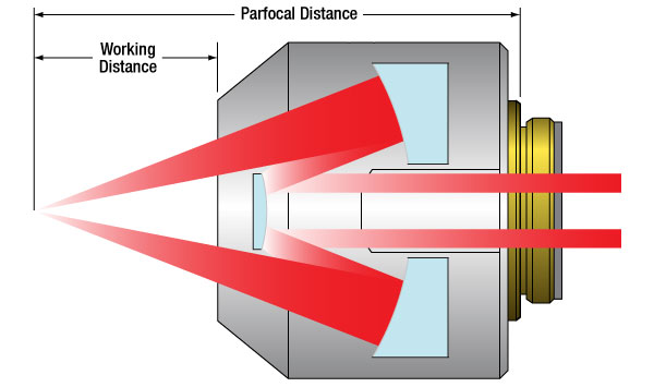
Click to Enlarge
Figure G1.1 This diagram illustrates the working distance and parfocal distance for reflective objectives with infinite back focal length.
- Reflective Objectives with 15X, 25X, or 40X Magnification
- Back Focal Length: Infinity
- UV-Enhanced Aluminum or Protected Silver Coatings
- RMS (0.800"-36) Objective Threading
These reflective objectives are designed with infinite back focal length and are ideal components of an infinity-corrected optical system in combination with our tube lenses. We offer three magnifications as well as two different reflective coatings (see Table G1.2). They are RMS threaded (0.800"-36) for compatibility with most manufacturers' microscopes.
Click on the red Document icon (![]() ) next to the item numbers below to access the Zemax file download. Our entire Zemax Catalog is also available.
) next to the item numbers below to access the Zemax file download. Our entire Zemax Catalog is also available.
| Table G1.2 Specifications | |||||||
|---|---|---|---|---|---|---|---|
| Item # | LMM15X-UVV | LMM25X-UVV | LMM40X-UVV | LMM15X-P01 | LMM25X-P01 | LMM40X-P01 | |
| Mirror Coating | UV-Enhanced Aluminum (Rabs > 80% Over 200 nm - 20 µm) |
Protected Silver (Ravg > 97% Over 450 nm - 2 µm; Ravg > 95% Over 2 µm - 20 µm) |
|||||
| Magnificationa | 15X | 25X | 40X | 15X | 25X | 40X | |
| Numerical Aperture | 0.3 | 0.4 | 0.5 | 0.3 | 0.4 | 0.5 | |
| Focal Length | 13.3 mm | 8 mm | 5.0 mm | 13.3 mm | 8 mm | 5.0 mm | |
| Parfocal Distanceb | 63.3 mm | 45.0 mm | 30.0 mm | 63.3 mm | 45.0 mm | 30.0 mm | |
| Back Focal Length | Infinity | Infinity | Infinity | Infinity | Infinity | Infinity | |
| Design Tube Lens Focal Lengthc | 200 mm | 200 mm | 200 mm | 200 mm | 200 mm | 200 mm | |
| Entrance Pupil Diameterd | 8.0 mm | 6.4 mm | 5.1 mm | 8.0 mm | 6.4 mm | 5.1 mm | |
| Working Distanceb | 23.8 mm | 12.5 mm | 7.8 mm | 23.8 mm | 12.5 mm | 7.8 mm | |
| Field of View | 1.2 mm | 0.7 mm | 0.5 mm | 1.2 mm | 0.7 mm | 0.5 mm | |
| Resolutione | 1.1 μm | 0.8 μm | 0.7 μm | 1.1 μm | 0.8 μm | 0.7 μm | |
| Obscurationf | Secondary Mirror Only | 22% | 22% | 18% | 22% | 22% | 18% |
| Mirror and Spider Vanes | 26% | 26% | 24% | 26% | 26% | 24% | |
| Transmitted Wavefront Error | <λ/14 RMS at 200 nm | <λ/14 RMS at 450 nm | |||||
| Damage Threshold | Pulsed | 0.3 J/cm2 (355 nm, 10 ns, 10 Hz, Ø0.381 mm) | 1.0 J/cm2 (1064 nm, 10 ns, 10 Hz, Ø0.230 mm) | ||||
| Objective Threading | 0.800"-36 (RMS) | ||||||
| RMS Thread Depth | 4.7 mm | 4.5 mm | 4.7 mm | 4.7 mm | 4.5 mm | 4.7 mm | |

 Zoom
Zoom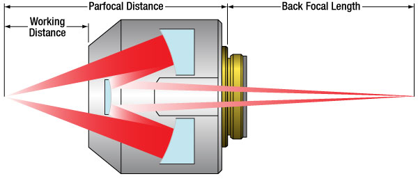
Click to Enlarge
Figure G2.1 This diagram illustrates the working distance, parfocal distance, and back focal length for reflective objectives with a finite back focal length.
- Reflective Objectives with 15X, 25X, or 40X Magnification
- Back Focal Length: 160 mm
- UV-Enhanced Aluminum or Protected Silver Coatings
- RMS (0.800"-36) Objective Threading
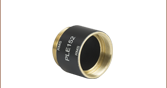
These reflective objectives are designed with a finite back focal length of 160 mm and are ideal for imaging applications where no refractive optical elements are desired. We offer three magnifications as well as two different reflective coatings (see Table G2.2 for details). They are RMS threaded (0.800"-36) for compatibility with most manufacturers' microscopes. The LMM40XF-UVV and LMM40XF-P01 objectives are shipped with an attached PLE152 Parfocal Length Extender. This hollow extender increases the parfocal length to 45 mm to match other parfocal length standards, such as those used by Olympus and Leica.
Click on the red Document icon (![]() ) next to the item numbers below to access the Zemax file download. Our entire Zemax Catalog is also available.
) next to the item numbers below to access the Zemax file download. Our entire Zemax Catalog is also available.
| Table G2.2 Specifications | |||||||
|---|---|---|---|---|---|---|---|
| Item # | LMM15XF-UVV | LMM25XF-UVV | LMM40XF-UVV | LMM15XF-P01 | LMM25XF-P01 | LMM40XF-P01 | |
| Mirror Coating | UV-Enhanced Aluminum (Rabs > 80% Over 200 nm - 20 µm) |
Protected Silver (Ravg > 97% Over 450 nm - 2 µm; Ravg > 95% Over 2 µm - 20 µm) |
|||||
| Magnification | 15X | 25X | 40X | 15X | 25X | 40X | |
| Numerical Aperture | 0.3 | 0.4 | 0.5 | 0.3 | 0.4 | 0.5 | |
| Focal Length | 13.3 mm | 8 mm | 5.0 mm | 13.3 mm | 8 mm | 5.0 mm | |
| Parfocal Distancea | 63.3 mm | 45.0 mm | 45.0 mmb | 63.3 mm | 45.0 mm | 45.0 mmb | |
| Back Focal Lengtha | 160 mm | 160 mm | 160 mmb | 160 mm | 160 mm | 160 mmb | |
| Entrance Pupil Diameterc | 8.0 mm | 6.4 mm | 5.1 mm | 8.0 mm | 6.4 mm | 5.1 mm | |
| Working Distancea | 23.8 mm | 12.5 mm | 7.8 mm | 23.8 mm | 12.5 mm | 7.8 mm | |
| Field of View | 1.2 mm | 0.7 mm | 0.5 mm | 1.2 mm | 0.7 mm | 0.5 mm | |
| Resolutiond | 1.1 μm | 0.8 μm | 0.7 μm | 1.1 μm | 0.8 μm | 0.7 μm | |
| Obscuratione | Secondary Mirror Only | 22% | 22% | 18% | 22% | 22% | 18% |
| Mirror and Spider Vanes | 26% | 26% | 24% | 26% | 26% | 24% | |
| Transmitted Wavefront Error | <λ/14 RMS at 200 nm | <λ/14 RMS at 450 nm | |||||
| Damage Threshold | Pulsed | 0.3 J/cm2 (355 nm, 10 ns, 10 Hz, Ø0.381 mm) | 1.0 J/cm2 (1064 nm, 10 ns, 10 Hz, Ø0.230 mm) | ||||
| Objective Threading | 0.800"-36 (RMS) | ||||||
| RMS Thread Depth | 4.7 mm | 4.5 mm | 4.7 mm | 4.7 mm | 4.5 mm | 4.7 mm | |