 Products Home

Capturing and Sharing Insights
Having the right information can save hours of work and frustration, but a lot of this valuable knowledge is not found in textbooks, taught in classes, or easily located by searching online sources. Much of this knowledge is gained through experience and trapped in the minds and lab notebooks of people working in the world of photonics.
Thorlabs is on a mission to collect these tips, tricks, guidelines, and practical techniques into a book of knowledge we call Insights. Click on the following links or browse the tabs on this page to read the Insights we have recorded as of today. This collection is always growing, so check back soon to see what new Insights have been added.
The Field of Photonics
- What is photonics?
Alignment of Optical Components
- What is a procedure for correcting a laser's beam pointing angle?
- How are two mirrors used to align a laser beam along a different path?
- What is the required spacing between two beam-steering mirrors?
Beam Expanders
- What is an example of a do-it-yourself Keplerian beam reducer?
- Can expanding a laser beam effectively create a smaller beam size?
- Does it matter whether a beam expander or reducer has a Keplerian or Galilean design?
Best Lab Practices
- Clamping Forks: Tip for Maximizing the Holding Force
- Optical Tables: Clamping Forks and Distortion of the Table's Surface
- Washers: Using Them with Optomech
- Electrical Signals: AC vs. DC Coupling
- Fiber Collimators: Tip for Mounting with Adapter
- How are the large mounting holes (counterbores) at the middle of a translation stage used?
- Is fast access to all mounting slots on a linear translation stage possible?
- What are some first steps to improving power measurements of low-power optical signals?
Collimation
- Does collimated light maintain a constant beam diameter out to infinity?
- Is the beam spot output by a collimating lens an image of the lamp or LED source?
Design Elements of Thorlabs' Products
- Do translation stages isolate mounted components from vibrations transmitted through the adjuster?
- Post Holders: Rectangular Channel in the Inner Bore
- Bases: For Stability Orient the Side with the Undercut Down
Fiber Optics
- When does NA provide a good estimate of the fiber's acceptance angle?
- Why is MFD an important coupling parameter for single mode fibers?
- Does NA provide a good estimate of beam divergence from a single mode fiber?
- What factors affect the amount of light coupled into a single mode fiber?
- Is the max acceptance angle constant across the core of a multimode fiber?
Imaging
- Does the condenser's NA affect the microscope's resolution?
- How does Köhler illumination work in microscopy?
Integrating Spheres
- Ultraviolet and Blue Fluorescence Emitted by Integrating Spheres
- Sample Substitution Errors
Lasers
- Are collimated beams always emitted parallel to the laser's axis?
- Quantum and Interband Cascade Lasers (QCLs and ICLs): Operating Limits and Thermal Rollover
- HeNe Lasers: Handling and Mounting Guidelines
- Beam Size Measurement Using a Chopper Wheel
- Can the thin-lens equation be used with laser light?
Lens Mounts
- Can C-mount and CS-mount cameras and lenses be used with each other?
- Do Thorlabs' scientific cameras need an adapter?
- Why can the FFD be smaller than the distance separating the camera's flange and sensor?
Motion Control
- How can a manual translation stage be motorized?
- Recording Position from Digital Micrometers
Off-Axis Parabolic (OAP) Mirrors
- Why use a parabolic mirror instead of a spherical mirror?
- Benefit of an Off-Axis Parabolic Mirror
- The Off-Axis Angle of an OAP Mirror
- Focus Collimated Light / Collimate Light from a Point Source Using an OAP Mirror
- Locating the Optical and Focal Axes of an OAP Mirror
- Paired OAP Mirrors Can Relay an Image and Make the Beam Accessible
- Mounting and Aligning an OAP Mirror
- Directionality of OAP-Mirror-Based Reflective Collimators
Optical Isolators and the Faraday Effect
- How can the strength of a material's Faraday effect be measured?
- What is needed to determine the direction and magnitude of the Faraday rotation angle?
Photodiodes
- How does wavelength affect rise time?
Polarization-Maintaining (PM) Fiber
- Does PM fiber preserve every input polarization state?
- How does polarization-maintaining fiber preserve linearly polarized light?
- What limits the extinction ratio (ER) of light output from PANDA and bow-tie PM fibers?
- What is beat length and why is it often specified for PM fiber, instead of polarization extinction ratio?
- Are polarization-maintaining fibers with stress rods affected by operating temperature?
Polarized Light
- Labels Used to Identify Perpendicular and Parallel Components
- How is the polarization ellipse related to the polarization state?
- How is a Poincaré sphere useful for representing polarization states?
- Can the extinction ratio of a polarizing component be measured using an unpolarized light source?
- Can a linearly polarized light source be used to measure the extinction ratio of a polarizing optic?
Reflective Elements
- Is there a rule for choosing the mirror's diameter based on the laser beam's diameter?
- How does alignment affect the beam path through a retroreflector?
- Why coat the backsides of solid prism retroreflectors with metal?
- Does the angle of incidence affect the output beam power from a corner-cube retroreflector?
Software and Writing Programs to Control Devices
- DM713 Digital Micrometer: LabVIEW and C# Programming References
Video Insights
- How to Align a Laser
- Optical Power Meter Parameter Setup for Improved Accuracy
- How to Motorize a Manual Translation Stage
- Tips for Bolting Post Holders to Optical Tables, Bases, and Breadboards
- How to Align an Optical Isolator
- Align a Linear Polarizer's Axis to be Vertical or Horizontal to the Table
- Cleave a Large-Diameter Silica Fiber Using a Hand-Held Scribe
- Measure the Insertion Loss of a Fiber Optic Component
- Create Circularly Polarized Light Using a Quarter-Wave Plate (QWP)
- Align a Linear Polarizer 45° to the Plane of Incidence
- Align Fiber Collimators to Create Free Space Between Single Mode Fibers
- Setting Up a TO Can Laser Diode (Viewer Inspired)
- Setting Up a Pigtailed Butterfly Laser Diode (Viewer Inspired)
- Distinguish the Fast and Slow Axes of a Quarter-Wave Plate
- Visual Studio® Project Setup and C# Programming - Kinesis® BBD300 Series Controller
- Build a Polarimeter to Find Stokes Values, Polarization State (Viewer Inspired)
- Raster Scan Using Visual Studio® and C# Programming- Kinesis® BBD300 Series
- Align an Off-Axis Parabolic (OAP) Mirror to Collimate a Beam (Viewer Inspired)
- Camera Setup and Image Acquisition Using Visual Studio® and C# Programming
- Align FiberPorts on a FiberBench (Viewer Inspired)
- Working with KF (QR) Vacuum Flange Components
- Mounting your Optomech: Bases, Post Holders, and Posts
- Use Laser Speckle to Find the Beam Focus
- Python® Automation of a Power Meter and Rotation Mount (Viewer Inspired)
- Working with CF Vacuum Flanges
- Calibrate a Spatial Light Modulator (SLM) for Phase Delay (Viewer Inspired)
- Collimate a Laser with a Shear-Plate Collimation Tester (Viewer Inspired)
- PM Fiber Coupling Methods to Align Incident Polarization (Viewer Inspired)
- Herriott Cell Setup and Configuration (Viewer Inspired)
- Collimate Light from an LED
- Build a Solar Imaging Telescope with Tracking Capability
- How Light’s Incident Angle Affects Transmission & Finding Brewster’s Angle
What is Photonics?
|
Photonics is the study and use of light. The word photonics is based on a “photon”, which is a single particle of light. This is similar to electronics where the electrons are single particles of charge that make up electric current. In photonics, the photons are single particles of energy that make up light. The amount of energy provided by a photon depends on the color (wavelength). For example, a laser pointer that outputs 1 mW of red (640 nm) light provides Light is generated by a variety of sources. Some come from nature, like the sun, fire, or bioluminescence (lightning bugs). Manufactured sources include light bulbs, LEDs, and lasers. Much like wires are used to transport electric current, photonics uses optical fiber to transport light from one location to another. |
Similar to electronics using resistors and capacitors to modify the current flow through a circuit, photonics uses optics like lenses, mirrors, and prisms to direct and modify light paths. Almost all analysis of light is done with the same measurement equipment used in electronics, but a device is required to first convert the photons into electrical current. Common uses for photonics are to measure distance (laser radar), transmit/receive information (telecommunications), image objects that are difficult to see by the eye alone (microscopes / endoscopes / borescopes), and create sensors such as the amount of oxygen in the blood (pulse oximeters) and the quality of the air around us (particle size and trace gas detection). |
Date of Last Edit: Apr. 20, 2022
Insights into Techniques for Aligning and Routing Laser Beams
Scroll down to read about motivations, techniques, and rules for aligning and routing collimated laser beams.
- What is a procedure for correcting a laser's beam pointing angle?
- How are two mirrors used to align a laser beam along a different path?
- What is the required spacing between two beam-steering mirrors?
What is a procedure for correcting a laser's beam pointing angle?
Pitch (tip) and yaw (tilt) adjustments provided by a kinematic mount can be used to make fine corrections to a laser beam's angular orientation or pointing angle. This angular tuning capability is convenient when aligning a collimated laser beam to be level with respect to a reference plane, such as the surface of an optical table, as well as with respect to a particular direction in that plane, such as along a line of tapped holes in the table.
Click to Enlarge
Figure 2: The beam can be aligned to travel parallel to a line of tapped holes in the optical table. The yaw adjustment on the kinematic mount adjusts the beam angle, so that the beam remains incident on the ruler's vertical reference line as the ruler slides along the line of tapped holes.
Click to Enlarge
Figure 1: Leveling the beam path with respect to the surface of an optical table requires using the pitch adjustment on the kinematic laser mount (Figure 2). The beam is parallel to the table's surface when measurements of the beam height near to (left) and far from (right) the laser's front face are equal.
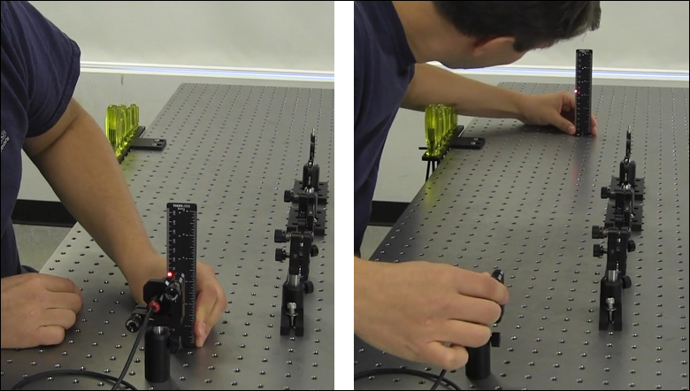
Video Clip 3: The pointing angle of a laser beam from a PL202 collimated laser package was corrected using the pitch (tip) and yaw (tilt) adjusters on the laser's KM100 kinematic mount, and horizontal and vertical features on a BHM1 ruler. The resulting beam travels parallel to the optical table's surface, along a line of tapped holes.
Before Using the Mount's Adjusters
First, rotate each adjuster on the kinematic mount to the middle of its travel range. This reduces the risk of running out of adjustment range, and the positioning stability is frequently better when at the center of an adjuster's travel range.
Then, make coarse corrections to the laser's height, position, and orientation. This can be done by adjusting the optomechanical components, such as a post and post holder, supporting the laser. Ensure all locking screws are tightened after the adjustments are complete.
Level the Beam Parallel to the Table's Surface
Leveling the laser beam is an iterative process that requires an alignment tool and the fine control provided by the mount's pitch adjuster.
Begin each iteration by measuring the height of the beam close to and far from the laser (Figure 1). A larger distance between the two measurements increases accuracy. If the beam height at the two locations differs, place the ruler in the more distant position. Adjust the pitch on the kinematic mount until the beam height at that location matches the height measured close to the laser. Iterate until the beam height at both positions is the same.
More than one iteration is necessary, because adjusting the pitch of the laser mount adjusts the height of the laser emitter. In Clip 3 for example, the beam height close to the laser was initially 82 mm, but it increased to 83 mm after the pitch was adjusted during the first iteration.
If the leveled beam is at an inconvenient height, the optomechanical components supporting the laser can be adjusted to change its height. Alternatively, two steering mirrors can be placed after the laser and aligned using a different procedure. Steering mirrors are particularly useful for adjusting beam height and orientation of a fixed laser.
Orient the Beam Along a Row of Tapped Holes
Aligning the beam parallel to a row of tapped holes in the table is another iterative process, which requires an alignment tool and tuning of the mount's yaw adjuster.
The alignment tool is needed to translate the reference line provided by the tapped holes into the plane of the laser beam. The ruler can serve as this tool, when an edge on the ruler's base is aligned with the edges of the tapped holes that define the line (Figure 2).
The relative position of the beam with respect to the reference line on the table can be evaluated by judging the distance between the laser spot and vertical reference feature on the ruler. Vertical features on this ruler include its edges, as well as the columns formed by different-length rulings. If these features are not sufficient and rulings are required, a horizontally oriented ruler can be attached using a BHMA1 mounting bracket.
In Clip 3, when the ruler was aligned to the tapped holes and positioned close to the laser, the beam's edge and the ends of the 1 mm rulings coincided. When the ruler was moved to a farther point on the reference line, the beam's position on the ruler was horizontally shifted. With the ruler at that distant position, the yaw adjustment on the mount was tuned until the beam's edge again coincided with the 1 mm rulings. The ruler was then moved closer to the laser to observe the effect of adjusting the mount on the beam's position. This was iterated as necessary.
Want additional Insights on beam alignment?
Watch the full video.
Date of Last Edit: Oct. 12, 2020
How are two mirrors used to align a laser beam along a different path?
The first steering mirror reflects the beam along a line that crosses the new beam path. A second steering mirror is needed to level the beam and align it along the new path. The procedure of aligning a laser beam with two steering mirrors is sometimes described as walking the beam, and the result can be referred to as a folded beam path. In the example shown in Clip 4, two irises are used to align the beam to the new path, which is parallel to the surface of the optical table and follows a row of tapped holes.
Click to Enlarge
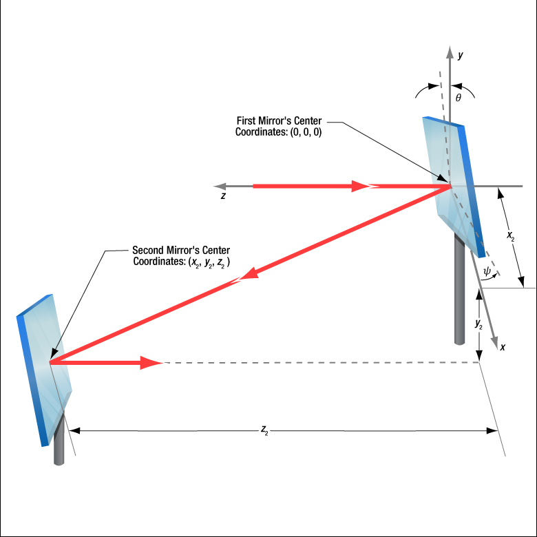
Figure 3: The beam reflected from Mirror 1 will be incident on Mirror 2, if Mirror 1 is rotated around the x- and y-axes by angles θ and ψ, respectively. Both angles affect each coordinate (x2 , y2 , z2 ) of Mirror 2's center. Mirror 1's rotation around the x-axis is limited by the travel range of the mount's pitch (tip) adjuster, which limits Mirror 2's position and height options.
Click to Enlarge
Figure 5: The adjusters on the second kinematic mirror are used to align the beam on the second iris.
Click to Enlarge
Figure 4: The adjusters on the first kinematic mirror mount are tuned to position the laser spot on the aperture of the first iris.
Video Clip 4: Two mirrors in KM100 kinematic mounts route the beam from a PL202 collimated laser package along the path defined by the two IDA25 irises. The beam is aligned when halos of laser light surround each iris' aperture and the laser spot is visible on the BHM1 ruler, which was placed behind the second iris to act as a viewing screen.
Setting the Heights of the Mirrors
The center of the first mirror should match the height of the input beam path, since the first mirror diverts the beam from this path and relays it to a point on the second mirror. The center of the second mirror should be set at the height of the new beam path.
Iris Setup
The new beam path is defined by the irises, which in Clip 4 have matching heights to ensure the path is level with respect to the surface of the table. A ruler or calipers can be used to set the height of the irises in their mounts with modest precision.
When an iris is closed, its aperture may not be perfectly centered. Because of this, switching the side of the iris that faces the beam can cause the position of the aperture to shift. It is good practice to choose one side of the iris to face the beam and then maintain that orientation during setup and use.
Component Placement and Coarse Alignment
Start by rotating the adjusters on both mirrors to the middle of their travel ranges. Place the first mirror in the input beam path, and determine a position for the second mirror in the new beam path (Figure 3). The options are notably restricted by the travel range of the first mirror mount's pitch (tip) actuator, since it limits the mirror's rotation (θ ) around its x-axis. In addition to the pitch, the yaw (tilt) of the first mirror must also be considered when choosing a position
After placing the second mirror on the new beam path, position both irises after the second mirror on the desired beam path. Locate the first iris near the second mirror and the second iris as far away as possible.
While maintaining the two mirrors' heights and without touching the yaw adjusters, rotate the first mirror to direct the beam towards the second mirror. Adjust the pitch adjuster on the first mirror to place the laser spot near the center of the second mirror. Then, rotate the second mirror to direct the beam roughly along the new beam path.
First Hit a Point on the Path, then Orient
The first mirror is used to steer the beam to the point on the second mirror that is in line with the new beam path. To do this, tune the first mirror's adjusters while watching the position of the laser spot on the first iris (Figure 4). The first step is complete when the laser spot is centered on the iris' aperture.
The second mirror is used to steer the beam into alignment with the new beam path. Tune the adjusters on the second mirror to move the laser spot over the second iris' aperture (Figure 5). The pitch adjuster levels the beam, and the yaw adjuster shifts it laterally. If the laser spot disappears from the second iris, it is because the laser spot on the second mirror has moved away from the new beam path.
Tune the first mirror's adjusters to reposition the beam on the second mirror so that the laser spot is centered on the first iris' aperture. Resume tuning the adjusters on the second mirror to direct the laser spot over the aperture on the second iris. Iterate until the laser beam passes directly through the center of both irises (Clip 4). If any adjuster reaches, or approaches, a limit of its travel range, one or both mirrors should be repositioned and the alignment process repeated.
If a yaw axis adjuster has approached a limit, note the required direction of the reflected beam and then rotate the yaw adjuster to the center of its travel range. Turn the mirror in its mount until the direction of the reflected beam is approximately correct. If the mirror cannot be rotated, reposition one or both mirrors to direct the beam roughly along the desired path. Repeat the alignment procedure to finely tune the beam's orientation.
If a pitch axis adjuster has approached a limit, either increase the two mirrors' separation or reduce the height difference between the new and incident beam paths. Both options will result in the pitch adjuster being positioned closer to the center of its travel range after the alignment procedure is repeated.
Want additional Insights on beam alignment?
Watch the full video.
Date of Last Edit: Oct. 22, 2020
What is the required spacing between two beam-steering mirrors?
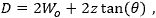
The required separation between two steering mirrors (Figure 6) depends on the slope of the beam reflected from the first mirror and the height difference between the two mirrors. Knowing the needed spacing can be important for blocking out space for a setup on a breadboard or optical table.
While it is tempting to perform a quick calculation using just the first mirror's pitch (tip) with respect to the incident beam, omitting the yaw (tilt) can result in a significant underestimate of the mirrors' required separation. In the following example, the spacing is calculated using the assumption that the entire mount is rotated around the post axis to provide yaw, while the mount's adjuster provides pitch (Figure 7). This approach is often used to initially position mirrors.
Click to Enlarge
Figure 7: Instead of using the yaw adjuster, the entire mount is often rotated around the post axis (left) to provide yaw during initial positioning. This rotates the mount with respect to the global x-, y-, z-axes and the incident beam. The mount's pitch adjuster tunes the mirror's pitch (right), changing the mirror's orientation with respect to the mount's x'-, y'-, and z'-axes. The above images show a KS2 mirror mount and a RMC position-maintaining collar.
Click to Enlarge
Figure 6: The first mirror reflects the incident beam towards the second mirror. The required spacing between the two depends on both the pitch and yaw of the first mirror. These KM100 mirror mounts have adjusters that can tune pitch and yaw over a ±4° range.
Click to Enlarge
Figure 9: These values were calculated using the setup described in Figure 8, except that a 1° pitch angle was assumed for the first mirror. These results demonstrate that decreasing the pitch increases the required separation between the first and second mirrors. However, this may be acceptable since stability improves when the adjusters are not extended to the limits of their travel ranges.
Click to Enlarge
Figure 8: In this example, the goal is to position the second mirror on the table, so that it intercepts the reflected beam when it is 0.5" lower (y2 = -0.5") than the incident beam. It is assumed the pitch on the first mirror is 4°, the maximum the mount's adjuster can provide. The entire mount is rotated around the post axis to change the first mirror's yaw. The mount's yaw adjuster is not used, since yaw angles >4° are of interest and this step does not involve fine-tuning the mirror's orientation.
Click to Enlarge
Figure 10: This plot views the table's surface from above, with the first mirror (star) at the origin. Curves labeled in the legend identify a few options for positioning a second mirror on the table to intercept the beam at a height (y2) that is 0.5" lower than at the first mirror. The required separation increases significantly as the first mirror's yaw angle increases, even when its pitch angle is held constant.
Applying Yaw and Pitch
Positioning beam steering mirrors is typically a two-step process. First the mirrors are placed in position and roughly oriented, then their orientations are finely tuned.
This example considers the first step and assumes different methods are used to adjust pitch and yaw. Since the required yaw angle is often too large for the mount's adjuster to provide, yaw is frequently provided by rotating the entire mount around the post axis (Figure 7, left). This changes the incident beam's angle with respect to the mount. Although the mount's yaw adjuster is not used, the pitch adjuster is used. It alters the orientation of the mirror with respect to both the incident beam and the rest of the mount (Figure 7, right).
The mirror's orientation is typically fine-tuned using the mount's pitch and yaw adjusters, without rotating the mount around the post axis. Using both adjusters has a different effect on the mirror's orientation than the approach described in this example.
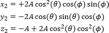
Points on the Reflected Beam
The first mirror's center is chosen as the origin of a fixed Cartesian coordinate system (Figure 7). The z-axis points back towards the source and is parallel to the incident beam. The y-axis is vertical and perpendicular to the table.
Points on the Reflected Beam
The first mirror's center is chosen as the origin of a fixed Cartesian coordinate system (Figure 2). The z-axis points back towards the source and is parallel to the incident beam. The y-axis is vertical and perpendicular to the table.
When the angles of rotation around the post and x'-axes are known ( and θ, respectively), points
 .
.
The variable A is a scaling factor: the larger its value, the larger the distance between the point and the mirror. In this example, the change in height (y2 ) is known and used to calculate values of x2 and z2 .
Example: Setting up Steering Mirrors
These equations can be useful when positioning a pair of steering mirrors, which are used to change beam height and direction. The center of the first mirror is set at the height of the incident beam, and the center of the second mirror is set at the height of the new beam path. The second mirror must intercept the reflected beam when its height equals that of the new beam path.
For this example, both beam paths are parallel to the optical table, but the new beam path is 0.5" lower than the incident beam path. The mirrors are secured in KM100 kinematic mounts, which are attached to the tops of posts secured in post holders (Figure 6). The mounts' pitch and yaw adjusters each have a limited ±4° tuning range, which is adequate for setting the initial pitch, but not yaw, of the mirror. The yaw between the incident beam and mirror is instead changed by rotating the entire mount around the post axis, which effectively eliminates the yaw tuning range limit.
Potential x2 and z2 coordinates of the second mirror are plotted in Figure 8 for different yaw angles of the first mirror. These values were calculated using the desired height change of the new beam path
Figure 10 plots the x2 and z2 coordinates of the second mirror as positions on the optical table. The perspective is from a point directly above the table, the first mirror's position is marked by a star, and the gray circles (guides for the eye) are concentric around it. The arrows indicate selected directions of the reflected ray, each corresponding to a different yaw angle. The curves labeled in the legend were calculated for different pitch angles and a constant -0.5" change in beam height. Comparing the curves with the gray circles illustrates that the necessary separation between the two mirrors increases significantly as the yaw angle increases. Larger separations are also required when the pitch angle is reduced.
Want additional Insights on beam alignment?
Watch the full video.
Date of Last Edit: Jan. 5, 2021
Insights into Beam Expanders
Scroll down to read about collimation and collimated beams. Collimation is used to reduce the divergence of light from narrowband laser sources with Gaussian beam profiles, as well as from broadband and white-light sources such as light emitting diodes (LEDs) and bulbs.
- What is an example of a do-it-yourself Keplerian beam reducer?
- Can expanding a laser beam effectively create a smaller beam size?
- Does it matter whether a beam expander or reducer has a Keplerian or Galilean design?
What is an example of a do-it-yourself Keplerian beam reducer?
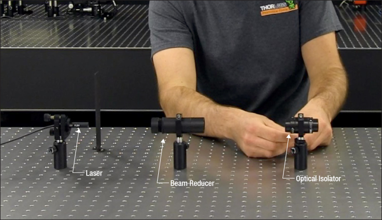
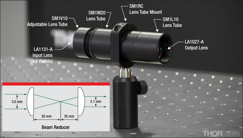
A beam reducer was designed and constructed for placement between a low-power continuous wave (CW) laser and a free-space optical isolator. The laser's wavelength was within the isolator's operating range, but the beam diameter exceeded the isolator's maximum specification. The design of the beam reducer was based on a Keplerian telescope and constructed using two positive lenses.
Click to Enlarge
Figure 1: A Keplerian beam reducer was designed and constructed to reduce the diameter of a laser beam, which was required to pass through an optical isolator's input and output apertures without clipping.
Click to Enlarge
Figure 2: This beam reducer was fabricated using two positive focal length lenses separated by the sum of their focal lengths. The reduction ratio equaled the focal length of the output lens divided by the focal length of the input lens. The labeled components (top) were used to assemble the beam reducer, and the output beam diameter was adjusted by measuring it while adjusting the SM1V10 lens tube length.
Beam Diameter Requirements
The laser source was a PL201, which outputs a CW and collimated beam with a wavelength of 520 nm and typical optical output power of 0.9 mW. At a distance 5 cm from the laser, a circle 3 mm in diameter would contain over 99% of the beam's power.
However, a specification for the free-space optical isolator
Reduction Ratio and Lens Choice
Beam reducer designs are often based on two-lens Keplerian or Galilean telescopes. Both approaches would provide similar performance in this application, but a Keplarian design was chosen to take advantage of the ease of using ray tracing geometry to graphically block out lens placements and show the output beam diameter (Figure 2, bottom).
Plano-convex lenses with 1" diameters, anti-reflective coatings, and positive focal lengths were chosen. Selecting lenses with large clear apertures compared with the beam diameter minimized aberrations, as did orienting the lenses so that their curved sides faced collimated beams and their flat sides faced the beam focus (Figure 2, bottom). In addition, 1" diameter optics are directly compatible with 1" diameter lens tubes and related accessories.
The target reduction ratio
Effect of Beam Reduction on Divergence Angle
A beam reducer shrinks the diameter of the beam waist but increases the divergence angle. Although the beam diameter would be 2.1 mm near the output face of the beam reducer, diffraction effects would cause the beam diameter to increase as it propagates. In this application, the beam diameter must be less than 2.7 mm in diameter after propagating across ~18 cm of free space to enter the isolator without clipping.
To investigate whether the reduced beam would meet the isolator's input diameter specification and travel through the isolator without clipping, the laser beam's waist diameter
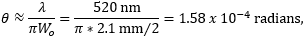
 is the wavelength of the laser light
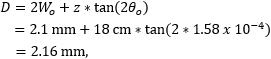
at the input to the isolator. The distance used in the equation was then increased
Construction
The ideal beam reducer design (Figure 2, bottom) assumes the input beam waist is one focal length (50 mm) away from the curved input side of the left lens. Under these conditions, the light focuses to a point that is one focal length away from the planar output side of the lens, as illustrated. When this input condition is not met, which is the case in this work, the focal point of the beam output by the first lens will not be exactly 50 mm away, and the diameter of the beam provided by the beam reducer will differ from the ideal calculated value. In order for the beam reducer to provide the specified beam diameter over the required distance, it may be necessary to adjust the spacing between the two lenses from the ideal design values. In this application, the housing was constructed to allow this spacing to be tuned.
The housing that secured and positioned the two lenses approximately 85 mm (3.4") apart from each other was constructed using lens tubes (Figure 2). As seen in this figure, the curved sides of the lenses faced the directions of the collimated light. A 3" tube was fabricated by attaching two fixed-length lens tubes, 1" (SM1L10) and 2" (SM1M20) together. The 35 mm lens was secured within the 1" lens tube. An adjustable lens tube (SM1V10), which held the 50 mm focal length lens, supplied the required additional length and allowed the distance between the two lenses to be optimized. The assembly was held in a lens tube mount (SM1RC) during the alignment of the isolator.
Want to see how this beam reducer was used?
Watch the full video.
Date of Last Edit: June 18, 2021
Can expanding a laser beam effectively create a smaller beam size?
Since a beam expander converts an input beam with a smaller waist and larger divergence into an output beam with a larger waist and smaller divergence, the output beam can have a smaller diameter far from the beam expander when compared with the input beam. The beam diameter does not remain constant with distance due to the effects of diffraction. As the beam divergence is higher for beams with smaller waists, using a beam expander to increase the waist diameter is a technique for reducing the rate at which the beam diameter increases as the beam propagates away from its waist. Beam expanders are often used to reduce beam divergence and ensure the beam diameter does not exceed a specified limit at distances far from the output beam waist.
Click to Enlarge
Figure 3: The input beam has a smaller waist diameter than the output beam. However, the diameter of the smaller input beam changes at a substantially higher rate than the larger output beam. Within the limited range shown above, the diameter of the input beam exceeds that of the output beam.
Click to Enlarge
Figure 4: A beam has a nearly constant divergence angle far from the beam waist. As described in the text, this angle
Beam Expanders (and Reducers)
Beam expanders (and beam reducers) accept a collimated beam with one waist diameter and provide a collimated beam with a different waist diameter. The expansion ratio, or magnification (m ),

relates the diameters of the beam waists before
Measuring the beam cross sections at the input and output beam waist locations can provide estimates of the waist diameters. The manufacturer often specifies the output beam waist location, but if it is not known, a measurement of the beam diameter close to the output of the beam expander can be used to approximate the waist diameter.
Beam Divergence
A laser beam's diameter is always smallest at its waist. Away from the waist, the beam diameter increases due to the effects of diffraction, and this rate of increase is the beam's angular divergence. Far from the beam waist, the divergence angle is approximately constant (Figure 4). An estimate of this divergence angle

can be calculated from the wavelength  )
)
The difference in the angular divergence of the beams input to and output from a beam expander or reducer can be estimated using the beam expansion ratio

in which θin and θout are the divergence angles of the input and output beams, respectively, far from their beam waists.
In the case of a beam expander
A beam reducer
Avoid Beam Clipping
The diameter of the output beam close to the beam expander is often a good approximation of the output beam waist diameter. Farther away, the beam diameter may have increased enough to cause beam clipping or other unintended effects. Calculating estimates of the beam diameter
at critical distances
Date of Last Edit: Aug. 23, 2021
Content improved by our readers!
Does it matter whether a beam expander or reducer has a Keplerian or Galilean design?
The design of the beam expander or reducer does not always matter to the application, but the choice can be influenced by factors such as the easier alignment and more intuitive design of the Keplerian devices and the compact dimensions of the Galilean devices. Additionally, a Keplerian device focuses the light between its two lenses and then outputs an inverted beam. A Galilean device maintains the orientation of the beam and provides the option to select lenses to reduce the amount of spherical aberration in the output beam.
Beam expanders and reducers are typically used only with collimated beams, rather than diverging beams, and these designs take their inspiration from Keplerian and Galilean telescopes. The magnification provided in both cases equals the focal length of the output lens divided by the focal length of the input lens.
Click to Enlarge
Figure 5: The simplest Keplerian beam expander or reducer includes two positive lenses. The focal lengths of Lens 1 and Lens 2 are f1 and f2, respectively. The lenses are separated by a distance equal to the sum of their focal lengths
Click to Enlarge
Figure 6: A basic Galilean beam expander or reducer includes a negative lens with focal length
Characteristics of the Keplerian Design
In the simplest Keplerian design, two positive lenses are separated by a distance equal to the sum of their focal lengths (Figure 5). A design based on the Keplerian telescope will never be shorter than the sum of the two lenses' focal lengths, and the output beam is inverted with respect to the input beam.
The beam comes to a focus between the two lenses. This provides the opportunity to spatially filter the beam. For example, a pinhole filter could be placed at the beam's focal point to improve beam quality. Away from the focus, the beam diameter expands as it approaches the output lens. To increase the diameter of the collimated beam provided by the output lens, it is necessary to move the output lens farther away from the focus. Since the distance between the focus and the output lens equals the focal length, this requires using a lens with a longer focal length.
The Keplerian design is typically not preferred for high-energy beams, such as the high-power pulsed laser beams used in some cutting and other manufacturing applications. Focusing pulses with nanosecond duration and optical powers around ~1 MW or higher, for example, can ionize the air and create a spark, which undesirably reduces the power of the pulse and can negatively affect the beam quality.
Characteristics of the Galilean Design
A basic Galilean telescope also includes two lenses, but one is negative while the other is positive (Figure 6). The lenses are positioned so that the distance between them equals the difference in their focal lengths, resulting in a more compact design than the Keplerian approach.
The Galilean approach can also be used to minimize the spherical aberration induced by the beam expander or reducer. All spherical lenses introduce spherical aberration, and one consequence is the spread of the beam focus along the optical axis. In the case of a positive spherical lens, parallel rays incident closer to the lens' outer perimeter focus to a point on the optical axis closer to the lens, compared with parallel rays incident near the lens' center. Since a negative spherical lens has the opposite effect, the negative lens in the Galilean design can be used to cancel out some of the spherical aberration induced by the positive lens.
When the device is used as a beam expander, the smaller-diameter beam is incident on the negative lens. The diverging beam provided by the negative lens increases in diameter as it approaches the positive lens, instead of focusing between the two lenses. This diverging beam can be described as having a virtual focus, which is located on the opposite side of the negative lens, as shown in Figure 6. Since the positive lens is one focal length
Expansion Ratio
Beam expanders and reducers are designed to accept and provide collimated beams. Although the beams are collimated, their diameters change as they propagate due to the effects of diffraction. Ideally, the input beam waist is positioned one focal length away from the input lens as shown in Figures 5 and 6. The output beam waist is then one focal length away from the output lens. If the input beam waist is not one focal length away from the input lens, the location of the output beam waist, the output beam waist diameter, and/or the divergence of the output beam may not match estimated values.
Both the beam's waist diameter
When the device includes two lenses, the formula for calculating the beam expansion ratio is the same for both Keplerian and Galilean designs. The beam expansion ratio equals the focal length of the output lens divided by the focal length of the input lens. The devices shown in Figures 5 and 6 are beam expanders when the light is incident on Lens 1, whose focal length is f1. In this case, the second lens (Lens 2) has focal length f2 and the beam expansion ratio

If the devices in Figures 5 and 6 are used as beam reducers, the light is incident from the opposite direction, upon Lens 2. Then, Lens 1 is the output lens, and the beam expansion ratio becomes m21 , which is f1 divided by f2.
Date of Last Edit: July 2, 2021
Insights into Best Lab Practices
Scroll down or click on one of the following links to read about practices we follow in the lab and things we consider when setting up equipment.
- Clamping Forks: Tip for Maximizing the Holding Force
- Optical Tables: Clamping Forks and Distortion of the Table's Surface
- Washers: Using Them with Optomech
- Electrical Signals: AC vs. DC Coupling
- Fiber Collimators: Tip for Mounting with Adapters
- How are the large mounting holes (counterbores) at the middle of a translation stage used?
- Is fast access to all mounting slots on a linear translation stage possible?
- What are some first steps to improving power measurements of low-power optical signals?
Clamping Forks: Tip for Maximizing the Holding Force
Click to Enlarge
Figure 2: More than half the total applied force (FTotal ) holds the object, since L1 > L2. The height of the left leg of this CL2 clamp is variable to compensate for the object's height. This allows the clamp's top surface and the mounting surface to be made parallel.**
Click to Enlarge
Figure 1: Less than half the total applied force (FTotal) holds the object, since L1 < L2. The clamp illustrated above is the CL5A.
Clamped objects can be fairly easy to move when the torqued screw in the clamp's slot is positioned too far from the object. Correct positioning of the screw protects clamped objects from being knocked out of position.
To maximize the clamping force, position the screw as close as possible to the object.**
This works since clamps like CL5A and CL2 (Figures 1 and 2, respectively) divide the torqued screw's applied force (FTotal) between two points.
Clamping force F2 is applied to the object. The value of F2 is a percentage of FTotal and depends on L1 and L2, as described below. The remainder (F1) of the total force is applied through the opposite end of the clamp.
The following equations can be used to calculate the two applied forces.
 |
Force Applied to the Other Contact Point: |  |
These equations show that the clamping force on the object increases as the distance between the object and screw decreases. The force supplied by the torqued screw is evenly divided between F1 and F2 when L1 and L2 are equal.
**Note that maximizing the clamping force also requires both the top surface of the clamp and the area it contacts on the object to be parallel with the mounting surface, as depicted in Figures 1 and 2.
If the tangent at the interface between the clamp and object is not parallel to the mounting surface, the force applied to the object will be divided between pressing it into and pushing it across the mounting surface. The force directed along the mounting surface may, or may not, be sufficient to translate the object.
To accommodate different object heights, clamps like the CL2 have one threaded, variable-length leg, which is shown on the left in Figure 2. The number of threads between the clamp and mounting surface should be adjusted to compensate for the height of the object and to keep the clamp's top surface level with the table.
Date of Last Edit: Dec. 4, 2019
Optical Tables: Clamping Forks and Distortion of the Table's Surface
Click to Enlarge
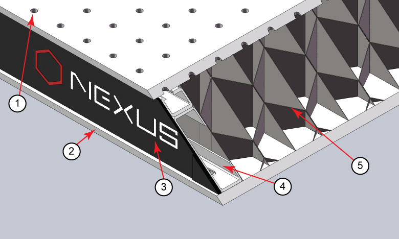
Figure 3: The construction of a Nexus table / breadboard includes a (1) top skin, (2) bottom skin, (3) side finishing trim, (4) side rails, and (5) honeycomb core. The stainless steel top and bottom skins are 5 mm thick.
Click to Enlarge
Figure 5: Torqueing the screw creates a force that pulls up on the table's top skin. The lifted skin tilts the mounting surface and can induce angular deviation of the object. This effect is exaggerated in the above image for illustrative purposes.
Click to Enlarge
Figure 4: A standard clamping fork, such as the CL5A, contacts the table along only one edge. The opposite edge is in contact with the object to be secured. A bridge forms between the two. The screw that applies the clamping force is not shown.

Click to Enlarge
Figure 6: The POLARIS-CA1/M clamping arm has a slot that accepts a mounting screw, a separate screw that applies a clamping force to an installed post, and identical top and bottom surfaces. Since a nearly continuous track around the surface of the clamping arm is in contact with the mounting surface, clamping arms cause negligible bridging effects.
Clamping forks are more rigid than the mounting surface of composite optical tables. It might be expected that the spine of the clamping fork would bend with the force exerted by the screw as the torque is increased. Instead, the screw will pull the skin of the table up and out of flat before the clamping fork deforms. Due to this, clamping forks should be used with care when securing components to optical tables. Clamping arms, which are discussed in the following, are alternatives to clamping forks that are less likely to deform the table's mounting surface.
Optical Table Construction
Optical tables and breadboards with composite construction (Figure 3) are designed to be rigid while providing vibration damping. The 5 mm thick, stainless steel top skin is manufactured to be flat, but a localized force can deform it. When the top skin is deformed, optical components will not sit flat, and optical system alignment and performance can be negatively affected.
Clamping Forks
Standard clamping forks are installed with one edge placed on the table's surface and the opposite edge on the object (Figure 4). Between these two edges, there is clearance between the bottom of the clamp and the surface of the table. This bridge makes it possible to use a single screw to both secure the clamp to the table and exert a holding force on the object.
When the clamp is secured by torqueing the screw, the screw pulls up on the top skin of the table (Figure 5).
As the torque on the screw increases, the top skin of the table rises. Not only does pulling up on the table surface risk permanently damaging the table, this can also disturb the alignment of the optical component the clamp is being used to secure. By lifting the table's skin, the mounting surface under the clamped object tilts.
Clamping Arms
Clamping arms, such as the POLARIS-CA1/M, shown in Figure 6, are designed to secure a post while minimally deforming the mounting surface.
The clamping arm in Figure 6 differs from clamping forks in two significant ways. One is the surface area that makes contact with the optical table, which is highlighted in red, and the other is the method used to secure the post.
The area in contact with the optical table makes a nearly continuous loop around the base of the clamp. The contact area is flat and flush with the table when the clamp is installed. The only break in the loop is a narrow slot in the vise used to grip the post.
This design uses two screws, instead of the clamping fork's single screw. One screw (not shown) secures the clamp to the table, and the other (indicated) is tightened to grip the post. Since one screw is not required to perform both tasks, it is not necessary for this clamping arm to form a bridge between the clamped object and the optical table.
Although the contact area is a loop, and not a solid surface, this clamp causes negligible distortion of the mounting surface. This is due to the open area inside the contact surface being narrow and surrounded by the sides of the clamp, which resist the force pulling up on the table.
Date of Last Edit: Dec. 4, 2019
Washers: Using Them with Optomech
Click to Enlarge
Figure 8: Install washers before inserting bolts into slots to protect the slot from damage. The rounded, smooth side of the washer should be placed against the slot, and the rough, flat side should be in contact with the bolt head. The smooth surface is designed to translate easily across the anodized surface, without harming it. The BA2 base is illustrated.
Click to Enlarge
Figure 7: The diameter of the washer is 35% larger than that of the bolt head. This results in over a six fold increase in overlap area with the slot of a BA2 base. By distributing the force of the bolt over a larger area, the washer help prevent gouging of the slot.
The head of a standard cap screw is not much larger than the major diameter of the thread (Figure 7). For example, a ¼-20 screw has a head diameter between 0.365" and 0.375" and the clearance hole diameter for the threads is 0.264".
When the screw is tightened directly through the clearance hole to secure the device, the force is applied to the edge of the through hole, often cutting into the material (Figure 7).
Once the material is permanently deformed, the screw head will want to fall back into the gouged groove, thereby moving the device back to that location when attempting to make fine adjustments.
A device with a circular through hole is not meant to translate around the screw thread so the deformation is not expected to be a problem.
However, a slot should provide the ability to secure the device anywhere along the length for the lifetime of the part. Using a washer distributes the force away from the slot edge to decrease the chance of deforming the slot and extending the lifetime of the part. Figure 7 illustrates the difference a washer can make. The contact area between the slot of a BA2 base and a 0.27" diameter cap screw is 0.010 in2. When a 0.5" diameter washer is used the contact area is 0.064 in2, which is over six times larger.
When using a Thorlabs washer, there are two distinct sides (Figure 8). One side is flat and rough and the other is curved and polished. The curved and polished side should be placed against the device, which has an anodized surface.
As the screw tightens, the screw head can force the washer to spin against the anodized coating.
If the flat side is pressed down against the anodization, the friction created by the rough flat side can scratch the anodized aluminum. However, if the curved side is facing down, the smooth surface has less friction leading to less scratches and extending the visual appearance of the device.
Date of Last Edit: Dec. 4, 2019
Electrical Signals: AC vs. DC Coupling
Click to Enlarge
Figure 9: The DC offset of a signal is its average value. Since the blue curve (AC Only) has an average amplitude of zero, it has a zero DC offset. The red signal (AC and DC) is identical to the blue, except the red signal has a non-zero AC offset. A DC coupling would pass the red signal unchanged. An AC coupling would remove the DC offset and attenuate low-frequency components of the signal.
When an instrument offers a choice between AC and DC coupled electrical inputs, it is not unusual for the DC coupling to be the better option for a modulated input signal.
AC and DC Couplings
AC and DC couplings are interfaces between the input signal and the rest of the instrument's circuitry.
A DC coupling, which is called a direct coupling, is essentially a wire connected to the signal input. This conductive coupling transmits all of the signal's frequency components, the DC as well as the AC. The red curve in Figure 9 has a non-zero DC component.
In an AC coupling, the key feature is a capacitor placed in series with the signal input. The capacitor functions as a high-pass filter and is sometimes called a blocking capacitor. AC couplings strongly attenuate the DC and low-frequency signal components. This capacitive coupling is used to remove the DC offset from the input signal, so that only AC components are passed. The blue curve in Figure 9 has only AC frequency components.
Use the DC Coupled Input When Possible
There are many reasons to prefer the DC coupled input. Its low-frequency response is very good, it allows the DC component of the signal to be monitored along with the AC, and it does not cause signal distortion since it does not affect the frequency content of the signal.
Use of the DC coupled input is recommended unless the DC offset is large or the filtering provided by the AC coupled input is required. One problem with a large DC offset is that it can reduce the resolution of the instrument to unacceptably low levels. In extreme cases, DC offsets can cause clipping and saturation effects.
Note that using the DC coupled input does not guarantee a signal free of distortion. Distortion can occur due to other reasons, such as insufficient device bandwidth or impedance mismatch at the termination.
Click to Enlarge
Figure 11: Some modulated signals, including the blue curve plotted above, have no DC component, but they do have non-negligible low-frequency components. When this signal is high-pass filtered by an AC coupling, the resulting signal is distorted. The green curve is one example of this.
Click to Enlarge
Figure 10: This frequency response magnitude plotted above models a capacitor-based high-pass filter. Its cutoff frequency (Fc) is 35 Hz, and it was used to filter the signal plotted in Figure 11. That signal has a repetition rate of 200 Hz.
Reasons to Use the AC Coupled Input
By rejecting the signal's DC component, AC coupling can reduce the total amplitude of the signal. This can increase the measurement resolution provided by the instrument, as well as overcome saturation and clipping problems. AC coupling provides good results when information is carried by high frequency signal components and low frequency components are not of interest. AC coupling can also be preferred when the application does not tolerate DC frequency signal components, as is the case for some telecommunications applications.
When Using the AC Coupled Input
If AC coupling is used, it is important to keep in mind that this coupling acts as a high pass filter and affects the frequency content of the signal.
As illustrated by Figure 10, this coupling does not just remove the DC offset, it can also attenuate low frequency components that may be of interest. Due to this, AC coupling can result in signal distortion. To illustrate the effects of high-pass filtering, Figure 11 plots a binary signal, with 200 Hz repetition rate, before and after it is filtered by the high-pass filter with 35 Hz cutoff frequency (Fc).
AC-coupled, digital telecommunications signals mitigate this problem by ensuring the signals are DC balanced, so that they have no DC offset. If the signals were not DC balanced, a series of ones could cause a sustained high signal level. This would introduce a non-zero DC level that would cause the signal to be affected by the capacitive filtering. The result could be bit errors due to high states being incorrectly read as low states.
Date of Last Edit: Dec. 4, 2019
Fiber Collimators: Tip for Mounting with Adapters
Click to Enlarge
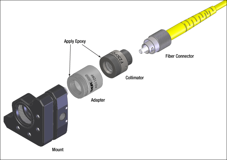
Figure 12: The components shown above are joined using threaded interfaces. Since unscrewing the fiber connector could unintentionally loosen connections between the other components, Thorlabs suggests applying epoxy to the other two interfaces to immobilize them.
Fiber collimators are often used to introduce light into an optical setup from a fiber coupled source. Thorlabs offers a variety of fiber collimator packages, some only provide a smooth barrel (like the triplet collimators) and others have a metric thread at the end of the barrel (like the asphere collimators).
For both packages, Thorlabs typically suggests the use of an adapter with a nylon tipped set screw that holds the barrel against a two line contact.
Adapters for the external thread are available (AD1109F) that allow the user to thread the fiber collimator into a mount.
However, the use of these adapters results in a stack up of threaded interfaces (threaded fiber connector, threaded collimator, and threaded adapter). As a result, it is possible that unscrewing the fiber connector could inadvertently loosen another thread interface and create an unknown source of instability in the setup.
For this reason, Thorlabs suggests epoxying the threaded fiber collimators into the threaded mounts if that mounting mechanism is preferred.
Date of Last Edit: Dec. 4, 2019
How are the large mounting holes (counterbores) at the middle of a translation stage used?
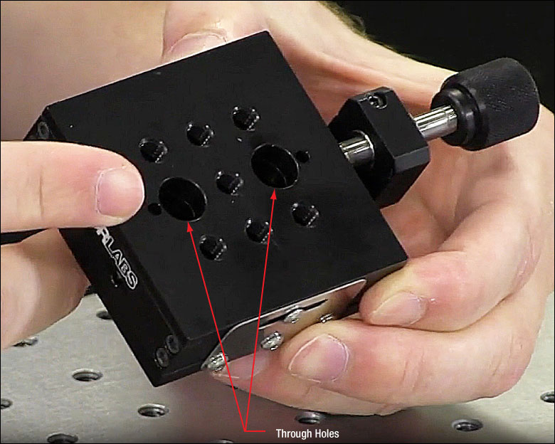
The mounting points used to secure some translation stages to a table or breadboard are located closer to the middle, rather than the perimeter, of the stage. Securing and releasing the stage from the mounting surface requires centering the top plate over the bottom (base) plate. When this is done, the oversized through holes on the top plate form a counterbore with the smaller through holes on the bottom plate.
Cap screws can then be inserted through the oversized holes in the top plate and screwed into the mounting surface to secure the stage. This is demonstrated using an MT1B linear translation stage. The stage can be released by loosening and removing the screws via the same holes.
Click to Enlarge
Figure 14: The two large through holes on the top plate of the stage provide access to the mounting points on the bottom of the stage.
Click to Enlarge
Figure 13: Through holes near the center of the stage's bottom plate are mounting points used to secure the stage to an optical table or breadboard.
Video Clip 1: The procedure for securing an MT1B linear translation stage to an optical table is demonstrated in this video clip.
Click to Enlarge
Figure 15: Each large through hole on the top surface of the stage provides the tip of a 3/16" (5 mm) ball driver access to the 1/4"-20 (M6) cap screws, which were previously inserted and used to secure the stage to the mounting surface.
Accessing the Mounting Points
The mounting points (Figure 13) are through holes located in the base plate, which is part of the stage's fixed world. The diameters of these through holes are large enough to pass the threads, but not the heads, of 1/4"-20 (M6) cap screws. Access to these mounting points is via the larger through holes (Figure 14) in the top plate, which is part of the stage's moving world.
However, accessing the mounting points requires aligning the top and bottom plates. The adjuster can be used to translate the top plate into alignment, so that each large through hole in the top plate is concentric with a smaller through hole in the bottom plate, forming counterbores. If a cap screw is inserted, threads first, into one of the through holes in the top plate, it should be possible to guide the threads through the hole in the bottom plate.
Secure the Stage First, then Mount Components
After the top and bottom plates are aligned, place the stage on the table or breadboard with the base plate in contact with the mounting surface. Align the counterbores with the threaded holes in the mounting surface, then insert a 1/4"-20 (M6) cap screw, from the top of the stage, into each through hole and then screw it into the table (Figure 15).
Since the top plate translates relative to the base plate, the top plate blocks access to the mounting points in general use. In addition, components mounted on the stage typically cover one or both of the through holes on the top plate. Due to this, it can be inconvenient to relocate the stage in the middle of an experiment. It is recommended that the stage be secured in an optimal location before mounting components on it.
Alternatively, a base plate like the MT401, which is designed for the MT stages, can be used to provide unobstructed mounting points at the perimeter of the stage. The stage is secured to the base plate as described here, and then the mounting slots on the base plate are used to secure the stage to a mounting surface.
Watch the Procedure Demonstrated
The procedure is demonstrated in the video clip (Clip 1), and the full video includes additional Insights on translation stages, including the procedure for replacing its adjuster screw with a motorized actuator.
Date of Last Edit: Sept. 8, 2020
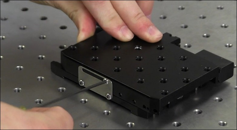
Is fast access to all mounting slots on a linear translation stage possible?
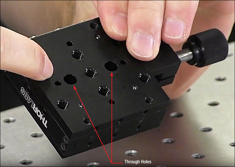
When a linear translation stage includes mounting slots at all four corners of the base plate, the position of the top plate usually blocks access to at least two of the mounting slots. A fast way to access all four slots, in pairs, is to retract the micrometer or actuator to expose two of the mounting slots, and then manually push the top plate into an extended position to expose the other two mounting slots. The top plate should then be held in the extended position by tightening the locking screw on the locking plate. This is demonstrated using an XR25P linear translation stage.
Click to Enlarge
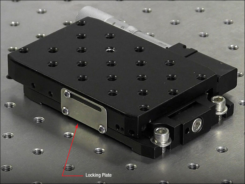
Figure 17: This perspective provides a view of the rectangular and slotted locking plate attached to the side of the stage opposite the micrometer. The image also shows that the top plate overhangs the two mounting slots at the back of the stage, blocking those slots when the slots at the front of the stage are exposed.
Click to Enlarge
Figure 16: When the micrometer is completely retracted, the two mounting slots on one side of the stage are accessible. Each mounting slot accepts a 1/4"-20 (M6) cap screw and washer. The two mounting slots on the other side of the stage are blocked by the top plate.
Video Clip 2: The procedure for securing an XR25P linear translation stage to an optical table is demonstrated in this video clip.
Click to Enlarge
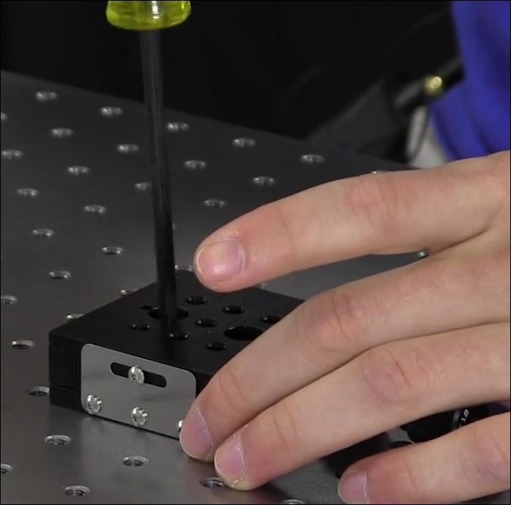
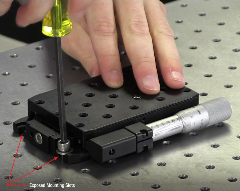
Figure 18: The top plate can be quickly pushed from a retracted position into an extended position, providing access to the other two mounting slots. Tightening the locking plate's screw with a 5/64" (2 mm) hex key will hold the top plate in position.
Retract the Micrometer to Access Two Slots
The four counterbored mounting slots used to secure these stages to an optical table or breadboard are integrated into the bottom (base) plate of these stages. Centering the top plate (moving world) over the base plate (fixed world) blocks access to all four mounting slots. Different pairs of mounting slots can be accessed when the top plate is retracted or extended.
To quickly access to all four slots, first retract the top plate using the micrometer or other adjuster. This exposes two of the mounting slots and makes it possible to secure or loosen a 1/4"-20 (M6) cap screw and its washer in each slot (Figure 16). As shown in Figure 17, the top plate overhangs and blocks the mounting slots on the other end of the stage in this position.
Push and Lock the Top Plate to Access Other Slots
If the top plate is in a retracted position and the base is held stationary, the top plate can be manually pushed into an extended position against the internal spring force. Do not let go of the top plate. If it is released, the spring force will propel the top plate backwards until it collides with the mechanical stop, which can damage the stage.
Push the top plate just far enough to expose the mounting slots on the back of the base plate, and then tighten the screw in the locking plate (Figure 18) to hold the top plate into position. With the top plate immobilized, 1/4"-20 (M6) screw and washer pairs can be installed in or removed from the newly accessible mounting slots.
Protect the Stage from Damage
When finished, hold the top plate to resist the spring force while loosening the screw in the locking plate. Slowly ease the top plate into its rest position to avoid causing a collision, whose mechanical shock can misalign the stage's components, affect the ball bearings, and introduce angular deviations to the stage's travel.
Watch the Procedure Demonstrated
The procedure is demonstrated in the video clip (Clip 2), and the full video includes additional Insights on translation stages, including the procedure for replacing its adjuster screw with a motorized actuator.
Date of Last Edit: Sept. 8, 2020
What are some first steps to improving power measurements of low-power optical signals?
Measurements of low-power optical signals can be improved by minimizing ambient light, blocking reflected and scattered light from reaching the power sensor (photosensor), ensuring the beam spot remains within the sensor's active area, optimally configuring the power meter's dynamic range, and performing the power meter's zeroing operation under ambient light conditions. The objective is to minimize the influence of spurious light sources on the power measurement, ensure that the sensor continuously measures the power delivered by the entire beam, and optimally configure the power meter for the experimental conditions.
Ambient Light
Ambient light is the light provided by all sources other than the optical system's light beam(s). In many cases, room lights are the greatest contributor to ambient light, but significant amounts can come from computer screens and other monitors, as well as light emitting diode (LED) indicators on instruments. A frustrating aspect of ambient light is that it can vary with the movement of the operator during the measurement, blinking of indicator lights, and screen display changes.
The effects of ambient light can include artificially inflating power readings, interfering with the detection of low-power signals, and saturating the sensor. When the sensor is saturated, the sensor outputs a signal near or at the maximum possible level. A sensor saturated by ambient light either cannot respond, or will respond poorly, to the additional power in the incident optical signal. The desired signal may also be undetectable if ambient light levels are low enough to avoid saturation, but high enough that the signal's contributed optical power is negligible in comparison.
Click to Enlarge
Figure 19: In the setup shown above, an SM1 lens tube is attached to the S130C optical power sensor, with the assistance of an SM1A29 thread adapter. The power sensor is positioned so that the exposed end of the lens tube nearly touches the transmission side of the nearest optical component. The lens tube helps isolate the power sensor from unwanted light. In a Video Insight, this setup was used to demonstrate a method for aligning a polarizer to be 45° to the plane of incidence.
Click to Enlarge
Figure 21: The beam spot can move across the power sensor due to alignment or normal operating conditions. The entire beam must be within the active area of the power sensor to accurately measure power. Circular movement of the beam spot during the measurement is illustrated above by the dashed-white circle. Ideally, the beam spot remains within the active area of the sensor (right). If the beam occasionally extends off of the power sensor (left), it can be hard to figure out that the associated power readings are artificially low.
Click to Enlarge
Figure 20: The front and back faces of the optic illustrated above are not parallel. Rotating the optic around the optical axis changes the direction of the transmitted beam. This type of situation can result in inaccurate measurements of optical power, as illustrated in (Figure 21).
Options for minimizing ambient light include turning off the room lights, installing the setup in a light-tight enclosure, covering monitors or turning screens to face away from the sensor, and / or turning off LEDs or covering them with black tape. Attaching a lens tube to the sensor housing as shown in Figure 19 can also be effective in reducing the ambient light incident on the power sensor.
Stray Light
Light beam(s) in the system can scatter, refract, and / or diffract from optics and mechanical housings in a setup, producing stray light. Stray light paths can be difficult to predict and block, since this light may interact multiple times with different optical elements and overlap the primary beam path. The effects of stray light on the measurement of the desired signal are similar to the effects of ambient light.
The best approach for blocking stray light depends on the beam trajectory and the setup, and often a combination of techniques are used. It is easiest to eliminate stray light that does not follow the beam path. Reflections can be directed away from the optical path by rotating optical surfaces away from normal incidence with the incident beam. However, this is only an option when the application is not sensitive to the optic's nonzero angle of incidence.
When the angle between the signal and stray light paths is reasonably large, a lens tube attached to the sensor (Figure 19) can block the stray light. If there is only a small angular difference between the stray light and signal paths, one option is to position an iris in front of the sensor to block the stray light while allowing the desired signal to pass through. Another option is to move the sensor farther away. With enough distance, the separation between the desired signal and the stray light will increase such that the stray light will either no longer be incident on the power sensor or will contribute negligibly to the power measurement.
Power Sensor Size and Beam Walk Allowance
The measured signal power will be artificially low if the diameter of the signal beam is larger than the active area of the power sensor. Note that the 1/e2 beam diameter, which is typically measured and specified for Gaussian beams, includes ~86% of the beam power. The diameter that encloses 99% of the beam power is a factor of ~1.5 larger than the 1/e2 diameter.
Ideally, the beam would be aligned so that it is centered on the active area of the sensor. If the beam is not aligned with the sensor's center, the risk of measurement errors increases. The power measurement will be low if the beam spot extends beyond the sensor's active area. If part of the beam overlaps with the active area, it may not be immediately obvious that there is a problem, since some signal power will be measured. Due to this, checking the overlap is recommended before taking measurements.
Imperfect overlap between the beam and power sensor might be a transient problem if the beam spot on the power sensor does not remain completely stationary during the measurement procedure. For example, the beam spot may wander if the measurement requires rotating an optical component around the optical axis (Figures 20 and 21). This is a particular concern if the front and back faces of the optic are not normal to the beam path. It may be possible to accommodate a moving beam spot by choosing a large-area power sensor.
Signal Within the Power Sensor's Dynamic Range
The sensor's dynamic range refers to the span of incident optical powers, minimum to maximum, compatible with the sensor. An accurate measurement requires the signal power to be within the sensor's dynamic range.
The noise floor typically defines the minimum detectable optical power level. The noise floor is the signal power reported by the power meter when absolutely no light is incident on the power sensor. The signal results from noise in the complete detector system, which includes the power sensor, power meter, cables, amplifiers, filters, and all other components. The incident signal will not be detected unless its optical power is sufficient to provoke a response exceeding the noise floor. Measurement accuracy may be poor when the signal response is close to the noise floor. A signal that is close to the noise floor has a low signal to noise ratio (SNR), which is the power in the desired signal divided by the noise power.
Power sensor manufacturers often specify maximum incident power levels below a threshold called the saturation intensity. Operating well below the saturation intensity threshold is recommended, since as the threshold is approached the sensor response becomes nonlinear and can result in power measurements that underestimate the power incident on the sensor. This can result in beam powers that unintentionally exceed applications' maximum operating power limits and is a significant concern. In the case of incident powers above the saturation intensity, the measurement reading is often a constant maximum value. One way to check for saturation conditions is to increase the signal power slightly while monitoring the power reading. If the reading remains constant, or changes much less than expected, it is likely that the sensor is saturated.
Zero the Power Meter to Ambient Light Levels
Set the zero value with the desired signal blocked from reaching the sensor, but without covering the power sensor. This can be done by blocking the signal at the source using an integrated shutter, if there is one, or by placing a beam block directly in front of the source. It is important that the beam block is not placed too close to the sensor, since during the zeroing procedure the power sensor should be exposed to the full ambient light level that will be present during the measurement. When this is done, the contribution of the ambient light will be subtracted from the measurement. If the sensor is covered while being zeroed, the ambient light power will be added to the measurement of signal power.
Date of Last Edit: May 16, 2022
Insights into Collimating Light from Different Types of Light Sources
Scroll down to read about collimation and collimated beams. Collimation is used to reduce the divergence of light from narrowband laser sources with Gaussian beam profiles, as well as from broadband and white-light sources such as light emitting diodes (LEDs) and bulbs.
- Does collimated light maintain a constant beam diameter out to infinity?
- Is the beam spot output by a collimating lens an image of the lamp or LED source?
Does collimated light maintain a constant beam diameter out to infinity?
Ideally, collimated light would have a constant diameter from the lens out to infinity, but no physical collimated beam maintains exactly the same diameter as it propagates. The collimated beam's divergence, which is the rate at which the beam's diameter changes, depends on the properties of both the light source and the collimator. Due to this, the collimated beam from a broadband-wavelength source, such as a lamp or light emitting diode (LED), behaves differently than the collimated beam from a narrowband-wavelength source, like a laser.
Click to Enlarge
Figure 1: If a broadband-wavelength source, like a lamp or LED, is placed one focal length
Click to Enlarge
Figure 3: The input parameters in Figure 2 create a collimated output beam with a waist located a distance one focal length (50 mm) from the lens. Note that this figure's scale is larger than the scale in Figure 2. Close to the beam waist  )
)
Click to Enlarge
Figure 2: A 632.8 nm laser source, which has a 5 µm diameter waist (Wo) and a 31 µm Rayleigh range (zR), is collimated by a 50 mm focal length (f ) lens.
Click to Enlarge
Figure 4: The input laser light better resembles a point source when it has a smaller beam waist (Wo), and therefore a shorter input Rayleigh range (zR). The collimated output beam has a Rayleigh range (zR') that depends on Wo , focal length, and wavelength. Increasing the focal length, or decreasing the wavelength, increases zR' and decreases the overall output beam divergence. The values plotted above were calculated for a 632.8 nm wavelength and a focal length of 50 mm. For comparison, values for a wavelength of 1550 nm and a focal length of 25 mm have also been calculated.
Collimated Lamp or LED Light
An ideal point source emits light uniformly in all directions, and a positive spherical lens placed one focal length
θ ~ d / f ,
of the collimated beam. The better the physical source resembles a single ideal point source, the lower the divergence angle of the collimated beam (Figure 1). The resemblance is closer when the physical source is very small, far away from the lens, or both.
A Lamp or LED as a Good-Enough Point Source
A physical source adequately resembles an ideal point source when the divergence of the collimated output beam meets the application's requirements. If the divergence is too large, one option is to increase the focal length of the collimating lens, so the source can be moved farther away. However, this can have the negative effect of reducing the amount of light collected by the lens and output in the collimated beam.
In Figure 1, light emitted from each point on the source fills the lens' clear aperture. Rays traced from different points on the source show the output beam's diameter is smallest at the lens, and the beam appears to diverge from the clear aperture of the lens. If light from each point on the source filled only a fraction of the lens' clear aperture, the beam waist would be displaced from the lens.
Laser Point Sources
The point source model can also be adapted for laser light, but in this case the source is defined as the input beam waist. The source size is the waist diameter
There are similarities between point source model adaptations for lasers and broadband sources. For example, laser sources should also be placed one focal length away from the lens to minimize the divergence of the collimated beam. In addition, the smaller the laser source (input beam waist diameter), the lower the collimated beam's divergence.
Unlike LEDs and lamps, laser sources do not emit light uniformly in all directions, although the laser light's divergence can be large. If the light comes from a single-wavelength laser, there's a good chance its intensity cross section resembles a Gaussian function. The collimated beam's behavior can then be described using Gaussian beam equations, and the equations describing beam divergence would need to include the wavelength.
Collimated Laser Light
The laser source's size helps determine the properties of the collimated beam. Size is typically referenced to the beam waist radius
 ,
,
in which () is the wavelength. When the input beam's waist and Rayleigh range are smaller, the collimated output beam has a lower divergence. (See Figures 2 and 3 for an example.) The divergence along the entire collimated beam can be reduced by shrinking the input source beam's waist diameter.
If the source waist is one focal length away from the lens, the collimated beam's waist is located one focal length away from the lens' opposite side. The beam's divergence increases with distance from the waist, and generalizations about the beam divergence can be made for regions close to and far from the waist.
Near the waist, the output beam best resembles an ideally collimated beam. In this region, the beam divergence is lowest, and the beam diameter stays close to the output beam waist diameter
 .
.
Some applications specify a distance  (~41%) larger than the waist diameter at a distance one Rayleigh range away from the beam. Examples of different relationships between zR and zR', the input and output beam's Rayleigh ranges, respectively, are plotted in Figure 4.
Far from the output beam waist
 .
.
Date of Last Edit: April 20, 2021
Is the beam spot output by a collimating lens an image of the lamp or LED source?
If a lens is placed one focal length away from sources like lamps or light-emitting diodes (LEDs), the lens will output light consisting of overlapping bundles of parallel rays that do not form an image but may form a beam spot (waist). Since each bundle of rays crosses the optical axis at a different angle, the intensity of the output light varies along the axis. The intensity is highest within the beam spot, where it may appear that the light comes to a focus. However, the rays in each bundle remain parallel, preventing the formation of an image. The location and diameter of the beam spot depends on the optical characteristics of the source and collimating lens, and both can be engineered to provide a beam spot that suits the application.
Click to Enlarge
Figure 6: When the source emits light over a wide range of angles, the light rays from each source spot are incident over the entire lens surface area. The lens outputs bundles of parallel rays, one bundle for each source point, but the beam spot is at the output surface of the lens, instead of being located one focal length away.
Click to Enlarge
Figure 5: Several factors provide a beam spot one focal length (f ) away from the lens. These include the symmetry of the emitted rays around the z-axis, and the limited lens surface area over which each cone of rays is incident. The lens outputs a single bundle of rays for each source point, and each bundle has a diameter smaller than the lens diameter. The overlapping ray bundles form the beam spot.
Click to Enlarge
Figure 7: A system of lenses can be used to form a beam spot wherever it is needed. In this case, the beam spot is located one focal length (fCD ) from the output side of the condenser lens. Since the rays emitted by each source point are parallel at the beam spot, no image is formed at the beam spot. Note that a scaled image of the source, where the rays from each point on the source intersect, is formed between the field and condenser lenses, one focal length (fFD ) away from the field lens. In this example, the light source is one focal length (fCL ) away from the collector lens.
Beam Spot, but No Image
The illustration in Figure 5 shows a light source on the left, which consists of a vertical stack of light-emitting points. While this is not a typical source, a system of lenses can be used to create an image of a source with these characteristics, as is discussed later.
The light rays from each point are spread over a limited range of angles (). This light is incident on a lens placed one focal length (f ) away. The lens outputs the light as bundles of parallel rays, one bundle for every light-emitting point on the source.
Each bundle of rays crosses the optical axis (z-axis) at a different angle. The angle for the light emitted from a particular light-emitting point on the source can be determined by first tracing a ray, from the point on the source, parallel to the z-axis, to the lens. From the endpoint of this ray, a second ray begins and crosses the z-axis one focal length away from the output side of the lens. In the figure, these are the rays at the center of each group and drawn with a thicker line.
The crossing of all of the parallel ray bundles provides a beam spot one focal length away from the lens. Here, the output beam has the smallest diameter and highest intensity. However, the spot does not include an image of the source, since the rays in each bundle are parallel to one another. All of the rays in each bundle would have to come back together, and intersect at a point, in order to form an image of the source point that emitted them.
There Is Not Always a Beam Spot
The lens in Figure 5 provides output light with a beam spot one focal length away from the lens for a few reasons. One is that the source is located one focal length away. Another is that the total group of rays emitted by the source are symmetric around the z-axis. In addition, the ray cone from each point intersects a limited region of the lens' surface area, so that each output bundle of rays has a relatively small diameter.
Figure 6 depicts a more typical white-light, or broadband source. Each point on the source emits rays over an angular range so wide that rays are incident upon the entire input face of the lens. When this occurs, the beam waist is located at the output surface of the lens.
Engineering a Beam Spot
Beam spots are useful for providing uniform illumination, since the light intensity is maximized and the beam spot does not include an image of the light-emitting structure of the source. When each point on the light source emits over a wide range of angles, and / or it is necessary to provide uniform illumination far from the lens, a system of lenses is often used.
A representative lens system is illustrated in Figure 7. The collector lens outputs bundles of parallel rays, and the beam spot is at the output surface of the lens, as in Figure 6. The field lens focuses each bundle of rays output by the collector lens. An upside-down, scaled image of the source's light emitting structure is formed one focal length away from both the field and condenser lenses. Since the light rays from this image are incident on the condenser lens over a limited region of the lens' input surface, the light output by this lens creates a beam spot one focal length away. The illumination provided by this beam spot is uniform, without an image of the source.
Date of Last Edit: May 7, 2021
Insights into Thorlabs' Design Details
Scroll down or click on one of the following links to read about design details, why they have been adopted, and how to take advantage of them.
- Do translation stages isolate mounted components from vibrations transmitted through the adjuster?
- Post Holders: Rectangular Channel in the Inner Bore
- Bases: For Stability Orient the Side with the Undercut Down
Do translation stages isolate mounted components from vibrations transmitted through the adjuster?
Translation stages can be designed to couple vibrations from the adjuster to the fixed world of the bottom (base) plate, away from the moving world of the top plate. Attaching the barrel clamp, which secures the adjuster, to the base plate minimizes the vibrations experienced by the mounted optomechanical components when the operator manipulates the adjuster.
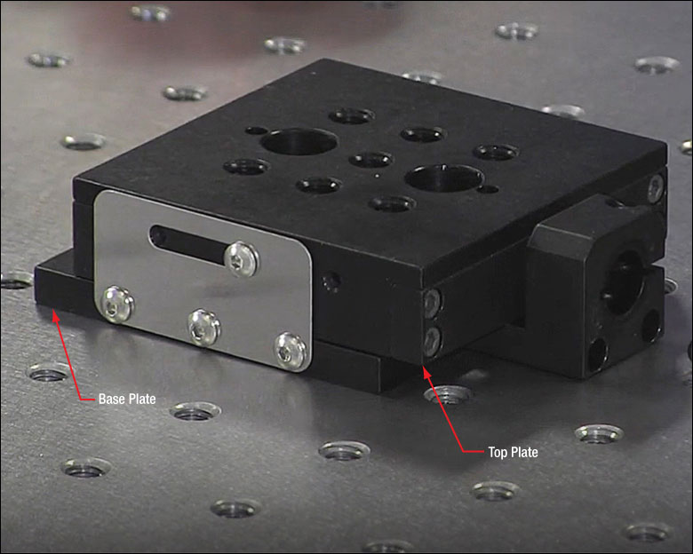
Click to Enlarge
Figure 2: The independence of the top plate from the barrel clamp is better illustrated with the adjuster screw removed, as shown above. The top plate is retracted and is higher than the base of the barrel clamp, which is attached to the base plate.
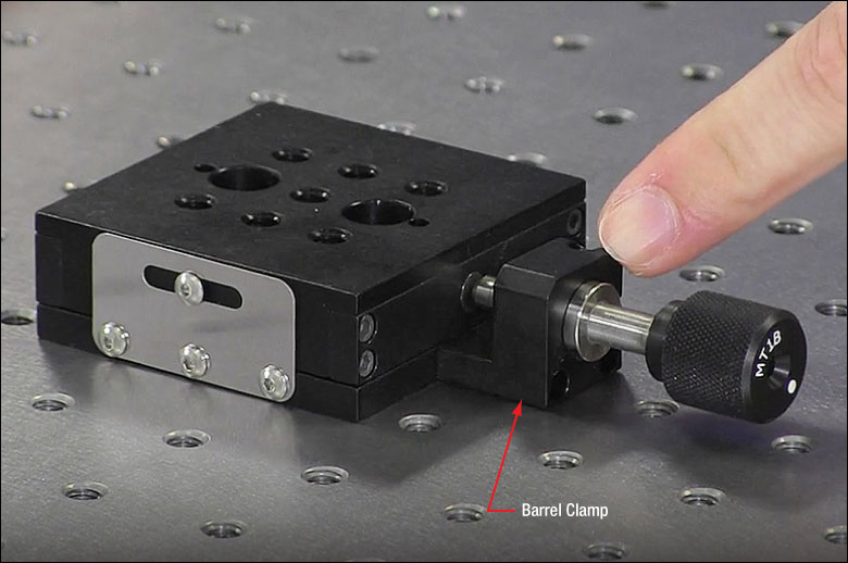
Click to Enlarge
Figure 1: The barrel clamp on the MT1B linear translation stage is indicated. Since the clamp is attached to the base plate, the top plate is isolated from vibrations arising from touching the adjuster screw.
Contact between Stage and Adjuster
Barrel clamps integrate manual adjusters or motorized actuators with translation stages (Figure 1). The barrel of the adjuster is gripped solidly and securely by the clamp, which creates a rigid mechanical contact that will efficiently couple vibrations from the adjuster to the clamp. Since the clamp is bolted directly to the base plate (Figure 2), vibrations from touching the adjuster will be routed to the fixed world of the stage. Those vibrations will be damped by the optical table or other mounting surface to which the stage is secured.
The only direct contact between the actuator and the stage's top plate, on which optomechanical components are mounted, occurs at a single point on the actuator's tip. Since this is not a rigid connection, it provides poor vibrational coupling between the actuator and the top plate. Similarly, contact points between the top and bottom plates are not rigid and do not efficiently transmit vibrations.
Want additional Insights on translation stages?
Watch a video that discusses mounting techniques and the procedure for replacing a stage's manual adjuster with a motorized actuator.
Date of Last Edit: Sept. 2, 2020
Post Holders: Rectangular Channel in the Inner Bore
Click to Enlarge
Figure 4: Top view. The three contact locations between the post and post holder, highlighted in red, prevent the post from translating or rotating around the x- or y-axes. Friction resists the post's translation and rotation around the z-axis.

Click to Enlarge
Figure 3: A channel with sharp edges is machined into the inner bore of Thorlabs' post holders.
Figure 5: A broach, such as the one illustrated above, has a row of teeth, the next taller than the previous. With the teeth in contact with the material, a machine pulls the broach across the surface. Each tooth removes a small amount of material, and the depth of the channel created by the broach equals the overall difference in tooth height.
All of Thorlabs' post holders include a channel, with straight parallel edges, running the length of the inner bore (Figure 3). Tightening the setscrew pushes the post against the two edges of the channel (Figure 4). Since the edges of the channel are separated by a wide distance, approximately half the inner diameter of the post holder, the seating of the post against the channel's edges is stable and repeatable.
Contact with the two edges of the channel eliminates four of the post's six degrees of freedom, since the edges block the post from translating along or rotating around either the y- or z-axis. In addition, the friction between the side of the post and the edges of the channel resists the post's movement along and around the x-axis, which are the post's two remaining degrees of freedom.
Without the channel in the inner bore, there would be a single line of contact between the post and post holder. The position of the post would not be stable, since the post would be free to rotate around the z-axis and shift along the y-axis.
Even if this instability resulted in submicron-scale unwanted shifts in each component's position in an optical setup, the cumulative effect could have a significant negative impact on system performance. In addition, more frequent realignment of the system could be required.
Broaching
The channel's edges must be straight and free of bumps and roughness to hold the post stable. These post holders have straight, sharp edges when examined on a micron scale. If the edges are not completely linear, the post might rock in the holder, and / or it may not be possible to repeatably position the post in the holder.
The smooth, straight edges of the channel are achieved using a machining process called broaching. A broach (Figure 5) resembles a saw whose teeth increase in height along its length.
As the broach is pulled along a surface, each tooth removes a small amount of material. The total depth of the channel cut by the broach equals to the overall difference in tooth height (H2 - H1 ).
Compared with other approaches for creating channels, broaching is preferred due to its ability to provide straight profiles while being compatible with high-volume production.
Date of Last Edit: Dec. 11, 2019
Bases: For Stability Orient the Side with the Undercut Down
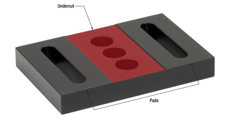
Click to Enlarge
Figure 7: This view of the bottom shows the undercut highlighted in red. By removing this material, the pads can be made maximally flat.
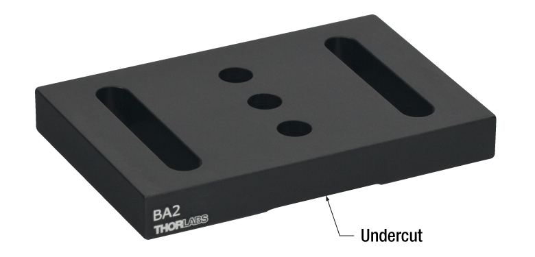
Click to Enlarge
Figure 6: For optimal stability, the base should be mounted with the undercut facing the optical table or breadboard.
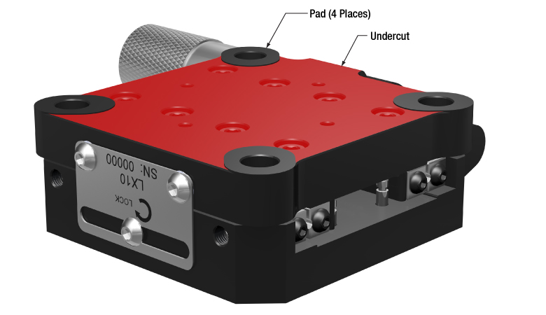
Click to Enlarge
Figure 9: Pads machined into Thorlabs' devices improve their stability when bolted in place. The pads are highly flat and project above the undercut region, which is highlighted red. The undercut limits the contact area with the table or breadboard.
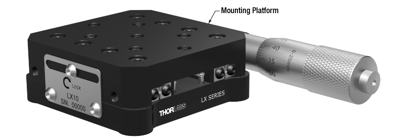
Click to Enlarge
Figure 8: The mounting platforms of stages and other devices do not feature pads.
An undercut is machined into the bottom surface of bases like the BA2 (Figures 6 and 7). The undercut creates feet, which are called pads. For maximum stability, the base should be oriented with its pads in contact with the table or breadboard.
The top surface of the base does not have an undercut and is the intended mounting surface for components.
Mounting the base upside down could result in the base rocking on the table or breadboard, or the base may exhibit other mechanical instability.
The Pads are Flatter than the Top Surface
The undercut is key to the flatness of the pads. The pads are machined flat after the undercut is made.
Friction heats the pads during the processing step that provides them with a maximally flat profile. By reducing the surface area of the pads, the undercut reduces the amount of heat generated during this step.
It is beneficial to minimize the heat generated during machining. Metal expands when heated, and the uneven heating that occurs during machining can distort the dimensions of the part. If the dimensions of the part are distorted during machining, the part can be left with high spots and other undesirable features after it cools. This can cause instability and misalignment when using the part.
Precision Instruments and Devices have Pads
Another example of a component with pads is the LX10 linear stage shown in Figures 8 and 9.
Date of Last Edit: Dec. 9, 2019
Insights into Fiber Optics
Scroll down or click on one of the links that follow to read about optical fiber, how it is used, and how to use them.
- When does NA provide a good estimate of the fiber's acceptance angle?
- Why is MFD an important coupling parameter for single mode fibers?
- Does NA provide a good estimate of beam divergence from a single mode fiber?
- What factors affect the amount of light coupled into a single mode fiber?
- Is the max acceptance angle constant across the core of a multimode fiber?
When does NA provide a good estimate of the fiber's acceptance angle?

Click to Enlarge
Figure 1: Rays incident at angles ≤θmax will be captured by the cores of multimode fiber, since these rays experience total internal reflection (TIR) at the interface between core and cladding. A requirement for TIR is that ncore > nclad .
Click to Enlarge
Figure 2: The behavior of the ray at the boundary between the core and cladding, which depends on their refractive indices, determines whether the ray incident on the end face is coupled into the core. The equation for NA can be found using geometry and the two equations noted at the top of this figure.
Numerical aperture (NA) provides a good estimate of the maximum acceptance angle for most multimode fibers, as shown in Figure 1. This relationship should not be used for single mode fibers.
Acceptance Angle and NA
In the ray model of light, a ray's angle of incidence determines whether or not it will be coupled into the fiber's core. The cutoff angle is the maximum acceptance angle (θmax ), which is related to the NA (Figure 1).
Rays with an angle of incidence ≤θmax are totally internally reflected (TIR) at the boundary between the fiber's core and cladding. As these rays propagate down the fiber, they remain trapped in the core.
Rays with angles of incidence larger than θmax refract at and pass through the interface between the core and cladding. This light may travel in the cladding for a while but is eventually lost from the fiber.
Geometry Defines the Relationship
The relationship between NA and θmax can be found using the geometry diagrammed in Figure 2. Snell's law was used at both interfaces, and the substitution sin(90°) = 1 was made. This geometry illustrates the most extreme conditions under which TIR will occur at the boundary between the core and cladding.
The refractive indices of the core and cladding, ncore and nclad , respectively, play a key role. In order for TIR to occur, ncore must be larger than nclad . The greater their difference, the larger the NA and maximum acceptance angle.
Angles of Incidence and Fiber Modes
When the angle of incidence is ≤θmax , the incident light ray is coupled into one of the multimode fiber's guided modes. Generally speaking, the lower the angle of incidence, the lower the order of the excited fiber mode. Lower-order modes concentrate most of their intensity near the center of the core. The lowest order mode is excited by rays incident normally on the end face.
Single Mode Fibers are Different
In the case of single mode fibers, the ray model in Figure 2 is not useful, and the calculated NA (acceptance angle) does not equal the maximum angle of incidence or describe the fiber's light gathering ability.
Single mode fibers have only one guided mode, the lowest order mode, which is excited by rays with 0° angles of incidence. However, calculating the NA results in a nonzero value. The ray model also does not accurately predict the divergence angles of the light beams successfully coupled into and emitted from single mode fibers. The beam divergence occurs due to diffraction effects, which are not taken into account by the ray model but can be described using the wave optics model. The Gaussian beam propagation model can be used to calculate beam divergence with high accuracy.
Date of Last Edit: Jan. 20, 2020
Why is MFD an important coupling parameter for single mode fibers?
Click to Enlarge
Figure 3 For maximum coupling efficiency into single mode fibers, the light should be an on-axis Gaussian beam with its waist located at the fiber's end face, and the waist diameter should equal the MFD. The beam output by the fiber also resembles a Gaussian with these characteristics. In the case of single mode fibers, the ray optics model and NA are inadequate for determining coupling conditions. The mode intensity (I ) profile across the radius ( ρ ) is illustrated.
As light propagates down a single mode fiber, the beam maintains a cross sectional profile that is nearly Gaussian in shape. The mode field diameter (MFD) describes the width of this intensity profile. The better an incident beam matches this intensity profile, the larger the fraction of light coupled into the fiber. An incident Gaussian beam with a beam waist equal to the MFD can achieve particularly high coupling efficiency.
Using the MFD as the beam waist in the Gaussian beam propagation model can provide highly accurate incident beam parameters, as well as the output beam's divergence.
Determining Coupling Requirements
A benefit of optical fibers is that light carried by the fibers' guided mode(s) does not spread out radially and is minimally attenuated as it propagates. Coupling light into one of a fiber's guided modes requires matching the characteristics of the incident light to those of the mode. Light that is not coupled into a guided mode radiates out of the fiber and is lost. This light is said to leak out of the fiber.
Single mode fibers have one guided mode, and wave optics analysis reveals the mode to be described by a Bessel function. The amplitude profiles of Gaussian and Bessel functions closely resemble one another [1], which is convenient since using a Gaussian function as a substitute simplifies the modeling the fiber's mode while providing accurate results.
Figure 3 illustrates the single mode fiber's mode intensity cross section, which the incident light must match in order to couple into the guided mode. The intensity (I ) profile is a near-Gaussian function of radial distance ( ρ ). The MFD, which is constant along the fiber's length, is the width measured at an intensity equal to the product of e-2 and the peak intensity. The MFD encloses ~86% of the beam's power.
Since lasers emitting only the lowest-order transverse mode provide Gaussian beams, this laser light can be efficiently coupled into single mode fibers.
Coupling Light into the Single Mode Fiber
To efficiently couple light into the core of a single-mode fiber, the waist of the incident Gaussian beam should be located at the fiber's end face. The intensity profile of the beam's waist should overlap and match the characteristics of the mode intensity cross section. The required incident beam parameters can be calculated using the fiber's MFD with the Gaussian beam propagation model.
The coupling efficiency will be reduced if the beam waist is a different diameter than the MFD, the cross-sectional profile of the beam is distorted or shifted with respect to the modal spot at the end face, and / or if the light is not directed along the fiber's axis.
References
[1] Andrew M. Kowalevicz Jr. and Frank Bucholtz, Beam Divergence from an SMF-28 Optical Fiber (NRL/MR/5650--06-8996) (Naval Research Laboratory, Washington, DC, 2006).
Date of Last Edit: Feb. 28, 2020
Does NA provide a good estimate of beam divergence from a single mode fiber?
Significant error can result when the numerical aperture (NA) is used to estimate the cone of light emitted from, or that can be coupled into, a single mode fiber. A better estimate is obtained using the Gaussian beam propagation model to calculate the divergence angle. This model allows the divergence angle to be calculated for whatever beam spot size best suits the application.
Since the mode field diameter (MFD) specified for single mode optical fibers encloses ~86% of the beam power, this definition of spot size is often appropriate when collimating light from and focusing light into a single mode fiber. In this case, to a first approximation and when measured in the far field,
 , , |
(1) |
is the divergence or acceptance angle (θSM ), in radians. This is half the full angular extent of the beam, it is wavelength )
| Rayleigh Range: | ||
 |
||
| Beam Radius at Distance z: | ||
 |
||
|
Figure 4: These curves illustrate the consequence of using NA to calculate the divergence (θSM ) of light output from a single mode fiber. Significant error in beam spot diameter can be avoided by using the Gaussian beam propagation model. This plot models a beam from SM980-5.8-125. The values used for NA and MFD were 0.13 and 6.4 µm, respectively. The operating wavelength was 980 nm, and the Rayleigh range was 32.8 µm. |
||
Gaussian Beam Approach
Although a diverging cone of light is emitted from the end face of a single mode optical fiber, this light does not behave as multiple rays travelling at different angles to the fiber's axis.
Instead, this light resembles and can be modeled as a single Gaussian beam. The emitted light propagates similarly to a Gaussian beam since the guided fiber mode that carried the light has near-Gaussian characteristics.
The divergence angle of a Gaussian beam can differ substantially from the angle calculated by assuming the light behaves as rays. Using the ray model, the divergence angle would equal sin-1(NA). However, the relationship between NA and divergence angle is only valid for highly multimode fibers.
Figure 4 illustrates that using the NA to estimate the divergence angle can result in significant error. In this case, the divergence angle was needed for a point on the circle enclosing 86% of the beam's optical power. The intensity of a point on this circle is a factor of 1/e2 lower than the peak intensity.
The equations to the right of the plot in Figure 4 were used to accurately model the divergence of the beam emitted from the single mode fiber's end face. The values used to complete the calculations, including the fiber's MFD, NA, and operating wavelength are given in the figure's caption. This rate of beam divergence assumes a beam size defined by the 1/e2 radius, is nonlinear for distances z < zR , and is approximately linear in the far field (z >> zR ).
The angles noted on the plot were calculated from each curve's respective slope. When the far field approximation given by Equation (1) is used, the calculated divergence angle is 0.098 radians (5.61°).
References
[1] Andrew M. Kowalevicz Jr. and Frank Bucholtz, Beam Divergence from an SMF-28 Optical Fiber (NRL/MR/5650--06-8996) (Naval Research Laboratory, Washington, DC, 2006).
Date of Last Edit: Feb. 28, 2020
Content improved by our readers!
What factors affect the amount of light coupled into a single mode fiber?
Click to Enlarge
Figure 6 Conditions which can reduce coupling efficiency into single mode fibers include anything that reduces the similarity of the incident beam to the optical properties of the fiber's guided mode.
Click to Enlarge
Figure 5 For maximum coupling efficiency into single mode fibers, the light should be an on-axis Gaussian beam with its waist located at the fiber's end face, and the waist diameter should equal the MFD.
Adjusting the incident beam's angle, position, and intensity profile can improve the coupling efficiency of light into a single mode optical fiber. Assuming the fiber's end face is planar and perpendicular to the fiber's long axis, coupling efficiency is optimized for beams meeting the following criteria (Figure 5):
- Gaussian intensity profile.
- Normal incidence on the fiber's end face.
- Beam waist in the plane of the end face.
- Beam waist centered on the fiber's core.
- Diameter of the beam waist equal to the mode field diameter (MFD) of the fiber.
Deviations from these ideal coupling conditions are illustrated in Figure 6.
These beam properties follow from wave optics analysis of a single mode fiber's guided mode [1].
The Light Source can Limit Coupling Efficiency
Lasers emitting only the lowest-order transverse mode provide beams with near-Gaussian profiles, which can be efficiently coupled into single mode fibers.
The coupling efficiency of light from multimode lasers or broadband light sources into the guided mode of a single mode fiber will be poor, even if the light is focused on the core region of the end face. Most of the light from these sources will leak out of the fiber.
The poor coupling efficiency is due to only a fraction of the light in these multimode sources matching the characteristics of the single mode fiber's guided mode. By spatially filtering the light from the source, the amount of light that may be coupled into the fiber's core can be estimated. At best, a single mode fiber will accept only the light in the Gaussian beam output by the filter.
The coupling efficiency of light from a multimode source into a fiber's core can be improved if a multimode fiber is used instead of a single mode fiber.
References
[1] Andrew M. Kowalevicz Jr. and Frank Bucholtz, Beam Divergence from an SMF-28 Optical Fiber (NRL/MR/5650--06-8996) (Naval Research Laboratory, Washington, DC, 2006).
Date of Last Edit: Jan. 17, 2020
Is the max acceptance angle constant across the core of a multimode fiber?
It depends on the type of fiber. A step-index multimode fiber provides the same maximum acceptance angle at every position across the fiber's core. Graded-index multimode fibers, in contrast, accept rays with the largest range of incident angles only at the core's center. The maximum acceptance angle decreases with distance from the center and approaches 0° near the interface with the cladding.
Click to Enlarge
Figure 7: Step-index multimode fibers have an index of refraction ( n ) that is constant across the core. Graded-index multimode fibers have an index that varies across the core. Typically the maximum index occurs at the center.

Click to Enlarge
Figure 9: Graded-index multimode fibers have acceptance angles that vary with radius ( ρ ), since the refractive index of the core varies with radius. The largest acceptance angles typically occur near the center, and the smallest, which approach 0°, occur near the boundary with the cladding
Click to Enlarge
Figure 8: Step-index multimode fibers accept light incident in the core at angles ≤|θmax | with good coupling efficiency. The maximum acceptance angle is constant across the core's radius ( ρ ). Air is assumed to surround the fiber.
Step-Index Multimode Fiber
The core of a step-index multimode fiber has a flat-top index profile, which is illustrated on the left side of Figure 7. When light is coupled into the planar end face of the fiber, the maximum acceptance angle (θmax ) is the same at every location across the core (Figure 8). This is due to the constant value of refractive index across the core, since the acceptance angle depends strongly on the index of the cladding.
Regardless of whether rays are incident near the center or edge of the core, step-index multimode fibers will accept cones of rays spanning angles ±θmax with respect to the fiber's axis.
Graded-Index Multimode Fibers
The core of a typical graded-index multimode fiber, shown on the right side of Figure 7, has a refractive index that is greatest at the center of the core and decreases with radial distance ( ρ ). The equation included below the diagram in Figure 9 shows that the radial dependence of the core's refractive index results in a radial dependence of the maximum acceptance angle and numerical aperture (NA). This equation also assumes a planar end face, normal to the fiber's axis that is surrounded by air.
Cones of rays with angular ranges limited by the core's refractive index profile are illustrated Figure 9. The cone of rays with the largest angular spread
Step-Index or Graded Index?
A step-index multimode fiber has the potential to collect more light than a graded-index multimode fiber. This is due to the NA being constant across the step-index core, while the NA decreases with radial distance across the graded-index core.
However, the graded-index profile causes all of the guided modes to have similar propagation velocities, which reduces the modal dispersion of the light beam as it travels in the fiber.
For applications that rely on coupling as much light as possible into the multimode fiber and are less sensitive to modal dispersion, a step-index multimode fiber may be the better choice. If the reverse is true, a graded-index multimode fiber should be considered.
References
[1] Gerd Keiser, Optical Fiber Communications (McGraw-Hill, New York, 1991), Section 2.6.
Date of Last Edit: Jan. 2, 2019
Insights into Imaging Systems
Scroll down or click on the following link for information about Köhler illumination and the importance of the condenser's numerical aperture to image resolution in microscopes.
- Does the condenser's NA affect the microscope's resolution?
- How does Köhler illumination work in microscopy?
Does the condenser's NA affect the microscope's resolution?
The condenser's numerical aperture (NA) strongly impacts a microscope's resolution, since the angular range of the light incident on the sample affects the angular range of light transmitted or reflected by the sample. According to a general rule for optimizing resolution, the condenser NA should be as least as large as the objective NA. In other words, the cone of light provided by the condenser should have an angular range that matches or exceeds that accepted by the objective lens.
Click to Enlarge
Figure 2: In epi-illumination microscopes, the objective provides the light that illuminates the sample. It also collects the light reflected and scattered from the sample. Due to this, and in contrast to the case illustrated in Figure 1, both the illumination and imaging angles depend only on the objective.
Click to Enlarge
Figure 1: In transmitted light microscopes, light from the light source is directed to the sample by the condenser optical system. The objective lens is used to collect the transmitted light. This collected light is then routed to create an image at a camera or eyepiece.
Click to Enlarge
Figure 3: Cones describe the light incident on a sample point from the condenser (left, gold), the light transmitted through the sample (right, yellow), and the range of light the objective can collect (right, orange). The cones' angles are measured from the optical axis. The angular ranges of the light cones incident on and transmitted by the sample are approximately the same
Condenser and Objective
In transmitted light microscopy, the condenser collects light from the source and illuminates the sample (Figure 1). The condenser optical system typically includes several optical elements, which can be aligned to provide uniform illumination of the sample plane. The objective lens is located on the opposite side of the sample plane and collects the light that is transmitted through the sample. This light is then routed to create an image at an eyepiece or camera.
Alternately, the microscope can be configured so the objective both illuminates and collects light from the sample (Figure 2). In this case, there is no separate condenser lens system.
Numerical Aperture
The condenser provides light to the sample plane over a range of different angles (Figure 3). A cone, drawn with its tip at a point on the sample and its base encircling the light from the condenser, can be used to quantify the range of incident angles
These angular ranges can be quantified by each lens' numerical aperture (NA),
NA = n sin(θ ),
which depends on the half-angle (θ ) of the cone, as well as the surrounding medium's refractive index (n ). The higher the NA, the wider the cone describing the angular range. This angle is measured from the optical axis.
As an example, when the objective lens has a 0.7 NA with air
Resolution
The resolution (δ ) of the microscope describes its ability to image two closely spaced points as a separable pair, instead of as a single point. A common equation,

used to estimate this minimum separation includes only the wavelength )
When NAcd ≤ NAobj , a modified version of the equation,
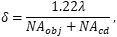
provides a better estimate and illustrates the importance of the condenser's NA to the resolution.
Date of Last Edit: June 9, 2021
How does Köhler illumination work in microscopy?
Click to Enlarge
Figure 4: An image of the source includes the structure of the light emitting elements (left). Köhler illumination avoids imaging the source to the sample or sensor planes and provides uniform illumination to the sample plane (right).
A multi-element microscopy system can be aligned to provide Köhler (Koehler) illumination, in which the light collected from a light source like a lamp or light emitting diode (LED) is imaged differently than the light collected from the sample. The light source is intentionally never imaged to the sample (object) plane or to the camera sensor. The sample plane is instead uniformly illuminated, typically over the broad range of angles required for high-resolution imaging. As a result, Köhler illumination prevents superimposing an image of the lamp or LED structure onto the camera sensor.
Image of the Light Source
An image of the light source at the sample plane would not uniformly illuminate the sample (Figure 4, left, for example), since the light-emitting structures are clearly visible in images of the source. Köhler illumination instead uniformly illuminates the sample plane (Figure 4, right) by providing the light to the sample plane as bundles of parallel rays. In addition, aligning the system to provide Köhler illumination prevents the light source from being imaged at the camera sensor, which would superimpose an image of the light-emitting structures onto the image of the sample.
Illumination Light Path
The illumination path begins with the light source and passes through the sample to the camera sensor. The video animation (Video 1, below) traces rays from an extended source, like a lamp or LED, through this light path.
Each of the multiple light-emitting points on the source radiate light over a range of angles. The collector lens gathers this light and transmits a beam whose maximum diameter is limited by the field stop. The light is then incident on the field lens, which forms an image of each source point at the aperture stop. The alignment of the source image at the aperture stop is critical, since the aperture stop is positioned at the front focal plane of the condenser lens.
The image of the source at the aperture stop provides light to the condenser lens, which transmits the light as bundles of parallel rays. Each bundle of rays originates from a unique point on the source image. The angle at which a particular bundle of rays is incident on the sample plane is larger when the source point is displaced farther from the optical axis. In other words, closing the aperture stop would reduce the range of illumination angles, as well as the illumination intensity at the sample plane.
Since an image of the source is at the front focal plane of the condenser lens, only bundles of parallel rays are incident on the sample plane. No source image is formed at the sample and the illumination is uniform.
Source light transmitted through the sample plane is imaged to the objective back focal plane, which is located between the objective and tube lenses. No image of the light source is formed on the camera sensor, which preserves image quality.
Imaging Light Path
The imaging path begins at the sample plane and ends at the camera sensor, and the video animation also traces rays through this light path. Each point on the sample is imaged to a point on the camera sensor.
Video 1: Optical elements in a transmission microscope, labeled on the left, are shown after they have been aligned to provide Köhler illumination. Under these conditions, as illustrated by the light rays traced through the illumination path in the animation, the sample plane is uniformly illuminated and images of the light source are not superimposed on the sample or camera sensor. In contrast, the light rays traced through the imaging path illustrate that the same optics do image the sample plane onto the camera sensor.
Date of Last Edit: June 18, 2021
Ultraviolet and Blue Fluorescence Emitted by Integrating Spheres
Click to Enlarge
Figure 1: Typical yields at each wavelength are around four orders of magnitude lower than the excitation wavelength. [4]
The spectral fluorescence yield relates the intensity of the fluorescence emitted within the integrating sphere with the intensity of the excitation wavelength. The yield is calculated by dividing the wavelength-dependent, total fluorescence excited over the entire interior surface of the sphere by the intensity of the light excitation.
Data were kindly provided by Dr. Ping-Shine Shaw, Physics Laboratory, National Institute of Standards and Technology, Gaithersburg, MD 20899, USA.
A material of choice for coating the light-diffusing cavities of integrating spheres is polytetrafluoroethylene (PTFE). This material, which is white in appearance, is favored for reasons including its high, flat reflectance over a wide range of wavelengths and chemical inertness.
However, it should be noted that integrating spheres coated with both PTFE and barium sulfate, which is an alternative coating with lower reflectance, emit low levels of ultraviolet (UV) and blue fluorescence when irradiated by UV light. [1-3]
Hydrocarbons in the PTFE Fluoresce
It is not the PTFE that fluoresces. The sources of the UV and blue fluorescence are hydrocarbons in the PTFE. Low levels of hydrocarbon impurities are present in the raw coating material, and pollution sources deposit additional hydrocarbon contaminants in the PTFE material of the integrating sphere during its use and storage. [1]
Fluorescence Wavelength Bands and Strength
Researchers at the National Institute of Standards and Technology (NIST) have investigated the fluorescence excited by illuminating PTFE-coated integrating spheres. The total fluorescence output by the integrating sphere was measured with respect to fluorescence wavelength and excitation wavelength. The maximum fluorescence was approximately four orders of magnitude lower than the intensity of the exciting radiation.
The UV and blue fluorescence from PTFE is primarily excited by incident wavelengths in a 200 nm to 300 nm absorption band. The fluorescence is emitted in the 250 nm to 400 nm wavelength range, as shown by Figure 1. These data indicate that increasing the excitation wavelength decreases the fluorescence emitted at lower wavelengths and changes the shape of the fluorescence spectrum.
As the levels of hydrocarbon contaminants in the PFTE increase, fluorescence increases. A related effect is a decrease of the light output by the integrating sphere over the absorption band wavelengths, due to more light from this spectral region being absorbed. [1, 3]
Impact on Applications
The UV and blue fluorescence from the PTFE has negligible effect on many applications, since the intensity of the fluorescence is low and primarily excited by incident wavelengths <300 nm. Applications sensitive to this fluorescence include long-term measurements of UV radiation throughput, UV source calibration, establishing UV reflectance standards, and performing some UV remote sensing tasks. [1]
Minimizing Fluorescence Effects
Minimizing and stabilizing the fluorescence levels requires isolating the integrating sphere from all sources of hydrocarbons, including gasoline- and diesel-burning engine exhaust and organic solvents, such as naphthalene and toluene. It should be noted that, while hydrocarbon contamination can be minimized and reduced, it cannot be eliminated. [1]
Since the history of each integrating sphere's exposure to hydrocarbon contaminants is unique, it is not possible to predict the response of a particular sphere to incident radiation. When an application is negatively impacted by the fluorescence, calibration of the integrating sphere is recommended. A calibration procedure described in [4] requires a light source with a well-known spectrum that extends across the wavelength region of interest, such as a deuterium lamp or synchrotron radiation, a monochromator, a detector, and the integrating sphere.
References
[1] Ping-Shine Shaw, Zhigang Li, Uwe Arp, and Keith R. Lykke, "Ultraviolet characterization of integrating spheres," Appl.Opt. 46, 5119-5128 (2007).
[2] Jan Valenta, "Photoluminescence of the integrating sphere walls, its influence on the absolute quantum yield measurements and correction methods," AIP Advances 8, 102123 (2018).
[3] Robert D. Saunders and William R. Ott, "Spectral irradiance measurements: effect of UV-produced fluorescence in integrating spheres," Appl. Opt. 15, 827-828 (1976).
[4] Ping-Shine Shaw, Uwe Arp, and Keith R. Lykke, "Measurement of the ultraviolet-induced fluorescence yield from integrating spheres," Metrologia 46, S191 - S196 (2009).
Date of Last Edit: Jan. 22, 2020
Sample Substitution Errors
Click to Enlarge
Figure 2: Measuring diffuse sample transmittance and reflectance as shown above can result in a distorted sample spectrum due to sample substitution error. The problem is that the reflectivity over the sample area is different during the reference and sample measurements.
Click to Enlarge
Figure 3: The above configuration is not susceptible to sample substitution error, since the interior of the sphere is the same for reference and sample measurements. During the reference measurement the light travels along (R), and no light is incident along (S). The opposite is true when a sample measurement is made.
Absolute transmittance and absolute diffuse reflectance spectra of optical samples can be found using integrating spheres. These spectra are found by performing spectral measurements of both the sample of interest and a reference.
Measurement of a reference is needed since this provides the spectrum of the illuminating light source. Obtaining the reference scan allows the spectrum of the light source to be subtracted from the sample measurement.
The light source reference measurement is made with no sample in place for transmittance data and with a highly reflective white standard reference sample in place for reflectance measurements.
Sample substitution errors incurred while acquiring the sample and reference measurement sets can negatively effect the accuracy of the corrected sample spectrum, unless the chosen experimental technique is immune to these errors.
Conditions Leading to Sample Substitution Errors
An integrating sphere's optical performance depends on the reflectance at each point on its entire inner surface. Often, a section of the sphere's inner wall is replaced by the sample when its transmittance and diffuse reflectance spectra are measured (Figure 2). However, modifying a section of the inner wall alters the performance of the integrating sphere.
Sample substitution errors are a concern when the measurement procedure involves physically changing one sample installed within the sphere for another. For example, when measuring diffuse reflectance (Figure 2, bottom), a first measurement might be made with the standard reference sample mounted inside the sphere. Next, this sample would be removed and replaced by the sample of interest, and a second measurement would be acquired. Both data sets would then be used to calculate the corrected absolute diffuse reflectance spectrum of the sample.
This procedure would result in a distorted absolute sample spectrum. Since the sample of interest and the standard reference have different absorption and scattering properties, exchanging them alters the reflectivity of the integrating sphere over the samples' surface areas. Due to the average reflectivity of the integrating sphere being different for the two measurements, they are not perfectly compatible.
Solution Option: Install Sample and Reference Together
One experimental technique that avoids sample substitution errors acquires measurement data when both sample and reference are installed inside the integrating sphere at the same time (Figure 3). This approach requires an integrating sphere large enough to accomodate the two, as additional ports.
The light source is located external to the integrating sphere, and measurements of the sample and standard reference are acquired sequentially. The specular reflection from the sample, or the transmitted beam, is often routed out of the sphere, so that only the diffuse light is detected. Since the inner surface of the sphere is identical for both measurements, sample substitution errors are not a concern.
Alternate Solution Option: Make Measurements from Sample and Reference Ports
If it is not possible to install both sample and standard references in the integrating sphere at the same time, it is necessary to exchange the installed sample. If this must be done, sample substitution errors can be removed by following the procedure detailed in [1].
This procedure requires a total of four measurements. When the standard sample is installed, measurements are made from two different ports. One has a field of view that includes the sample and the other does not. The sample of interest is then subsituted in and the measurements are repeated. Performing the calculations described in [1] using these measurements removes the sample substitution errors.
References
[1] Luka Vidovic and Boris Majaron, "Elimination of single-beam substitution error in diffuse reflectance measurements using an integrating sphere," J. Biomed.Opt. 19, 027006 (2014).
Date of Last Edit: Dec. 4, 2019
Insights into Lasers
Scroll down or click on one of the following links to read about operating lasers and tips for mounting them.
- Are collimated beams always emitted parallel to the laser's axis?
- QCLs and ICLs: Operating Limits and Thermal Rollover
- HeNe Lasers: Handling and Mounting Guidelines
- Beam Size Measurement Using a Chopper Wheel
- Can the thin-lens equation be used with laser light?
Are collimated beams always emitted parallel to the laser's axis?
A laser may not emit its beam parallel to the long axis of the laser package. This angular deviation is called the pointing angle (θp) and is described in Clip 1. Compensating for an angular deviation can be achieved when a kinematic mount with pitch (tip) and yaw (tilt) adjustments is used to position the laser.
Video Clip 1: The pointing angle (θp) is the angular deviation between the direction of the collimated laser beam (red arrow) and the long axis of the laser housing (dotted line). This axis is perpendicular to the front face of the collimator or collimated laser package.
Video Clip 2: Fitting a PL202 collimated laser package with an AD11NT adapter makes it possible to secure the laser in a KM100 mount that provides pitch (tip) and yaw (tilt) adjustment capability.
Angular Deviation
Several factors can result in angular deviation of the beam, including non-optimal seating of the laser in a mount, the laser cavity not being perfectly centered in the housing, and the deflection of the beam as it travels through optics integrated within the laser package. The compounded tolerances (tolerance stack up) result in a non-zero pointing angle.
When the laser has a cylindrical housing, this deviation can be measured by placing the laser in a V-groove mount, rotating the laser around its long axis, and recording the diameter of the circle traced by the laser spot. Maximum angular deviation is often specified for collimated laser packages.
Using a Kinematic Mount to Correct the Angle
One method to correct the angle of a laser beam is to secure the laser in a kinematic mount and use the mount's adjusters to tune the pitch and yaw of the laser.
In some cases, the kinematic mount is directly compatible with the outer diameter of the laser housing. Kinematic V-mounts, including those compatible with Ø1.5" posts, can be configured to accept a range of different housing diameters without the use of an adapter.
Other kinematic mounts have an inner bore with a fixed diameter. A variety of adapters, including some designed for cylindrical or SM-threaded components, are available to create compatibility between the outer diameter of the laser housing and the mounts' inner bore.
Attaching an Adapter
The procedure for using an AD11NT adapter to install a PL202 collimated laser package into a KM100 kinematic mount is demonstrated in Clip 2. Before attaching the adapter, pass the laser head through the bore of the kinematic mount, from back to front.
Because there is a stop integrated into the back plane of the mount's inner bore, it is necessary to attach the adapter on the side of the mount opposite the adjusters. The stop helps secure 1" diameter optics in the bore, but it also prevents the 1" diameter adapter from being inserted into the bore from the back of the mount.
The adapter includes nylon-tipped setscrews to secure the laser, and the mount also includes a nylon-tipped setscrew to secure the adapter. Nylon-tipped setscrews are chosen to securely grip the installed component without scratching or otherwise marring its surface.
Want additional Insights on correcting for the pointing angle?
Watch the full video.
Date of Last Edit: Oct. 12, 2020
QCLs and ICLs: Operating Limits and Thermal Rollover
Click to Enlarge
Figure 1: This example of an L-I curve for a QCL laser illustrates the typical non-linear slope and rollover region exhibited by QCL and ICL lasers. Operating parameters determine the heat load carried by the lasing region, which influences the peak output power. This laser was installed in a temperature controlled mount set to 25 °C.

Click to Enlarge
Figure 2: This set of L-I curves for a QCL laser illustrates that the mount temperature can affect the peak operating temperature, but that using a temperature controlled mount does not remove the danger of applying a driving current large enough to exceed the rollover point and risk damaging the laser.
The light vs. driving current (L-I) curves measured for quantum and interband cascade Lasers (QCLs and ICLs) include a rollover region, which is enclosed by the red box in Figure 1.
The rollover region includes the peak output power of the laser, which corresponds to a driving current of just under 500 mA in this example. Applying higher drive currents risks damaging the laser.
Laser Operation
These lasers operate by forcing electrons down a controlled series of energy steps, which are created by the laser's semiconductor layer structure and an applied bias voltage. The driving current supplies the electrons.
An electron must give up some of its energy to drop down to a lower energy level. When an electron descends one of the laser's energy steps, the electron loses energy in the form of a photon. But, the electron can also lose energy by giving it to the semiconductor material as heat, instead of emitting a photon.
Heat Build Up
Lasers are not 100% efficient in forcing electrons to surrender their energy in the form of photons. The electrons that lose their energy as heat cause the temperature of the lasing region to increase.
Conversely, heat in the lasing region can be absorbed by electrons. This boost in energy can scatter electrons away from the path leading down the laser's energy steps. Later, scattered electrons typically lose energy as heat, instead of as photons.
As the temperature of the lasing region increases, more electrons are scattered, and a smaller fraction of them produce light instead of heat. Rising temperatures can also result in changes to the laser's energy levels that make it harder for electrons to emit photons. These processes work together to increase the temperature of the lasing region and to decrease the efficiency with which the laser converts current to laser light.
Operating Limits are Determined by the Heat Load
Ideally, the slope of the L-I curve would be linear above the threshold current, which is around 270 mA in Figure 1. Instead, the slope decreases as the driving current increases, which is due to the effects from the rising temperature of the lasing region. Rollover occurs when the laser is no longer effective in converting additional current to laser light. Instead, the extra driving creates only heat. When the current is high enough, the strong localized heating of the laser region will cause the laser to fail.
A temperature controlled mount is typically necessary to help manage the temperature of the lasing region. But, since the thermal conductivity of the semiconductor material is not high, heat can still build up in the lasing region. As illustrated in Figure 2, the mount temperature affects the peak optical output power but does not prevent rollover.
The maximum drive current and the maximum optical output power of QCLs and ICLs depend on the operating conditions, since these determine the heat load of the lasing region.
Date of Last Edit: Dec. 4, 2019
HeNe Lasers: Handling and Mounting Guidelines
Click to Enlarge
Figure 3: The external housing of HeNe lasers is mechanically coupled to the components of the lasing cavity. Stress applied to the external housing can misalign and potentially fracture lasing cavity components, which can negatively impact the quality and power of the output laser beam (red arrow) or lead to laser failure
| 1. | High Reflector Optics | 7. | Anode |
| 2. | Gas Reservoir | 8. | Glass Laser Bore |
| 3. | Outer Housing | 9. | |
| 4. | Glass | 10. | Potting Compound |
| 5. | Glass-Metal Seal | 11. | Cathode |
| 6. | Output Coupling Optics |
HeNe lasers should be handled and mounted with care to protect them from damage.
Never apply a bending force to the laser housing. Stress applied to the laser's external housing can misalign or damage components in the laser cavity. This can:
- Affect the output beam quality.
- Result in reduced output power.
- Affect the beam pointing.
- Cause multimode effects.
Factory packaging protects the HeNe lasers from shocks and vibrations during shipping, but end users directly handle the bare laser housing. Due to this, HeNe lasers are in greater danger of experiencing dangerous stress during handling by the end user.
A result is that the primary cause of damage to HeNe lasers is rough handling after receipt of the laser. In extreme cases, shock and vibrations can shatter or fracture glass components internal to the laser.
To maintain the optimum performance of your HeNe laser, do not drop it, never use force when inserting it into fixture, and use care when installing it into mounts, securing it using cage components or ring accessories that grip the housing, transporting it, and storing it.
HeNe lasers will provide optimum performance over a long lifetime when they are handled gently.
Date of Last Edit: Dec. 4, 2019
Beam Size Measurement Using a Chopper Wheel
Click to Enlarge
Figure 5: The blade traces an arc length of Rθ through the center of the beam and has a angular rotation rate of  f. The chopper wheel shown is MC1F2.
Click to Enlarge
Figure 4: An approximate measurement of beam size can be found using the illustrated setup. As the blade of the chopper wheel passes through the beam, an S-curve is traced out on the oscilloscope.
Click to Enlarge
Figure 7: The diameter of a Gaussian beam is often given in terms of the 1/e2 full width.

Click to Enlarge
Figure 6: Rise time (tr ) of the intensity signal is typically measured between the 10% and 90% points on the curve. The rise time depends on the wheel's rotation rate and the beam diameter.
Camera and scanning-slit beam profilers are tools for characterizing beam size and shape, but these instruments cannot provide an accurate measurement if the beam size is too small or the wavelength is outside of the operating range.
A chopper wheel, photodetector, and oscilloscope can provide an approximate measurement of the beam size (Figure 4). As the rotating chopper wheel's blade passes through the beam, an S-shaped trace is displayed on the oscilloscope.
When the blade sweeps through the angle θ , the rise or fall time of the S-curve is proportional to the size of the beam along the direction of the blade's travel (Figure 5). A point on the blade located a distance R from the center of the wheel sweeps through an arc length (Rθ ) that is approximately equal to the size of the beam along this direction.
To make this beam size measurement, the combined response of the detector and oscilloscope should be much faster than the signal's rate of change.
Example: S-Curve with Rising Edge
The angle ftr )ftr )
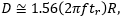
includes a factor of 1.56, which accounts for the portion of the beam measured between the 10% and 90% intensity points being smaller than the 1/e2 beam diameter.
Date of Last Edit: June 22, 2021
Content improved by our readers!
Can the thin-lens equation be used with laser light?
In the case of laser light, a modified thin-lens equation that takes diffraction into account is recommended instead of the conventional thin-lens equation. The modified equation, which models the laser light as Gaussian beams, is appropriate for many single-mode and fiber-coupled laser sources. In addtion, the equation can be adapted for use when the laser light does not have a perfect Gaussian intensity profile. [1]
Click to Enlarge
Figure 8: A thin lens, with focal length f , is shown inserted in a Gaussian beam. In the modified thin-lens equation, the object is the input beam's waist, located a distance s from the input side of the lens. The input beam's radius (W ) is Wo at its waist and maintains a similar radius over the Rayleigh range (±zR ). The image is the output beam's waist, located a distance s ' from the lens' output side. The output beam's radius (W ') is Wo' at its waist and remains nearly Wo ' over its Rayleigh range (±zR').
Click to Enlarge
Figure 10: Gaussian beam parameters such as the radius, W(z), and the wavefront's radius of curvature, R(z), are calculated using a distance, z, referenced to the beam's waist. The waist is always located at the origin.
Click to Enlarge
Figure 9: Key to the model are the relationships between the input and output beams at the lens. There, the beams have equal radii, and the beams' wavefront curvatures are related by the focal length of the lens. The wavefront' radius of curvature is flat (thick vertical line) at the waist and gradually becomes more spherical with increasing distance from the waist.
| Ray-Optics Thin-Lens Equation | ||||
| Conventional Thin-Lens Equation |  |
|||
| Gaussian Beam Equations | Lens System Relations | |||
| Beam Radius | 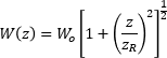 |
Beam Radii at Lens | 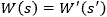 |
|
| Wavefront's Radius of Curvature |
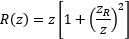 |
Wavefront Curvatures at Lens |
 |
|
| Rayleigh Range | |
Magnification (m ) |  |
|
| Gaussian Beam Thin-Lens Equations | ||||
| Modified Thin-Lens Equation | Input Beam Perspective | 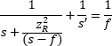 |
||
| Output Beam Perspective | 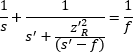 |
|||
| Magnification | 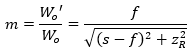 |
|||
Objects, and Images, and Laser Beams
The conventional thin-lens equation (table, top) is based on the ray optics model and uses the focal length (f ) of the lens to relate the distance
In the modified thin-lens equation, these distances refer to the separations between the lens and the input and output beam waists, respectively (Figure 8). The radius of a beam is smallest at its waist and increases with distance. A lens placed in the beam outputs a new beam with its own waist and divergence characteristics. The input beam waist radius (Wo ) is treated as the object size, and output beam waist radius (Wo' ) as the image size.
The modified thin-lens equation also includes either the input Rayleigh range
Modified Thin-Lens Equation
The incident and output light are assumed to propagate as Gaussian beams (Figure 9). The modified thin-lens equation was derived by relating the input and output beam properties (table, center) across the lens:
- The beam radii at the lens' input and output surfaces must be the same,
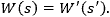
- The lens' focal length relates the radius of curvature (R ) of the wavefront incident upon the lens to the radius of curvature (R ') of the wavefront leaving the lens,
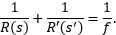
- Magnification (m ) is the ratio of the output and input beam waist radii (or diameters),

Note that the beam radius (W ) and wavefront's radius of curvature (R ) are calculated using the relative distance (z ) from the waist (Figure 10). There are two modifed thin-lens equations (table, bottom), since the form of the equation differs depending on whether the input beam parameters (zR and s ) or the output beam parameters (zR ' and s ') are known.
If the laser beam is not perfectly Gaussian, its Rayleigh range will be shorter than the Rayleigh range of an ideal Gaussian beam with the same waist radius. The ratio of the two values, M2 (M-squared), is often specified for laser beams. Multiply the beam's Rayleigh range by the M2 value, and then use this product as zR or zR ' in the modified thin-lens equation to find s ' or s , respectively.
Unique Behavior of Gaussian Beams
The behavior of Gaussian beams can be surprising, especially when compared with the predictions of the ray optics model and the conventional thin-lens equation.
For example, the conventional thin-lens equation (see table), predicts the image will appear at infinity when the object is placed at the lens' front focal point. However, for Gaussian beams, when the object beam waist is one focal length away from the input side of the lens, the image beam waist is one focal length away from the output side.
In another case, the conventional thin-lens equation predicts the image can be infinitely distant. But, if the beam is Gaussian with a nonzero Rayleigh range, the beam waist cannot be imaged to infinity. Instead, the maximum image beam waist distance,
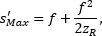
depends on the Rayleigh range of the input beam. For the image beam waist to appear at this distance, the object beam waist should be separated from the lens by a distance one Rayleigh range larger than the focal length,  )
)
References
[1] Sidney A. Self, "Focusing of spherical Gaussian beams," Appl.Opt. 22, 658-661 (1983).
Date of Last Edit: May 20, 2021
Insights into Mounting Lenses to Thorlabs' Scientific Cameras
Scroll down to read about using adapters to create compatibility between lenses and cameras of different mount types, with a focus on Thorlabs' scientific cameras.
- Can C-mount and CS-mount cameras and lenses be used with each other?
- Do Thorlabs' scientific cameras need an adapter?
- Why can the FFD be smaller than the distance separating the camera's flange and sensor?
Can C-mount and CS-mount cameras and lenses be used with each other?
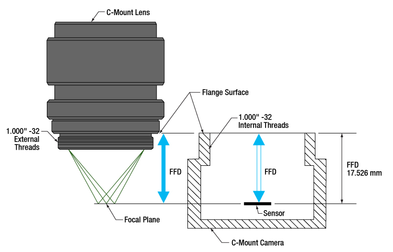
Click to Enlarge
Figure 1: C-mount lenses and cameras have the same flange focal distance (FFD), 17.526 mm. This ensures light through the lens focuses on the camera's sensor. Both components have 1.000"-32 threads, sometimes referred to as "C-mount threads".
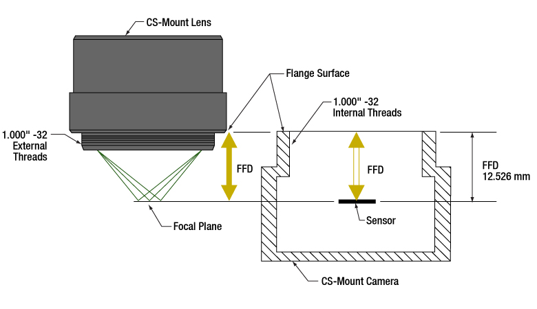
Click to Enlarge
Figure 2: CS-mount lenses and cameras have the same flange focal distance (FFD), 12.526 mm. This ensures light through the lens focuses on the camera's sensor. Their 1.000"-32 threads are identical to threads on C-mount components, sometimes referred to as "C-mount threads."
The C-mount and CS-mount camera system standards both include 1.000"-32 threads, but the two mount types have different flange focal distances (FFD, also known as flange focal depth, flange focal length, register, flange back distance, and flange-to-film distance). The FFD is 17.526 mm for the C-mount and 12.526 mm for the CS-mount (Figures 1 and 2, respectively).
Since their flange focal distances are different, the C-mount and CS-mount components are not directly interchangeable. However, with an adapter, it is possible to use a C-mount lens with a CS-mount camera.
Mixing and Matching
C-mount and CS-mount components have identical threads, but lenses and cameras of different mount types should not be directly attached to one another. If this is done, the lens' focal plane will not coincide with the camera's sensor plane due to the difference in FFD, and the image will be blurry.
With an adapter, a C-mount lens can be used with a CS-mount camera (Figures 3 and 4). The adapter increases the separation between the lens and the camera's sensor by 5.0 mm, to ensure the lens' focal plane aligns with the camera's sensor plane.
In contrast, the shorter FFD of CS-mount lenses makes them incompatible for use with C-mount cameras (Figure 5). The lens and camera housings prevent the lens from mounting close enough to the camera sensor to provide an in-focus image, and no adapter can bring the lens closer.
It is critical to check the lens and camera parameters to determine whether the components are compatible, an adapter is required, or the components cannot be made compatible.
1.000"-32 Threads
Imperial threads are properly described by their diameter and the number of threads per inch (TPI). In the case of both these mounts, the thread diameter is 1.000" and the TPI is 32. Due to the prevalence of C-mount devices, the 1.000"-32 thread is sometimes referred to as a "C-mount thread." Using this term can cause confusion, since CS-mount devices have the same threads.
Measuring Flange Focal Distance
Measurements of flange focal distance are given for both lenses and cameras. In the case of lenses, the FFD is measured from the lens' flange surface (Figures 1 and 2) to its focal plane. The flange surface follows the lens' planar back face and intersects the base of the external 1.000"-32 threads. In cameras, the FFD is measured from the camera's front face to the sensor plane. When the lens is mounted on the camera without an adapter, the flange surfaces on the camera front face and lens back face are brought into contact.

Click to Enlarge
Figure 5: A CS-mount lens is not directly compatible with a C-mount camera, since the light focuses before the camera's sensor. Adapters are not useful, since the solution would require shrinking the flange focal distance of the camera (blue arrow).
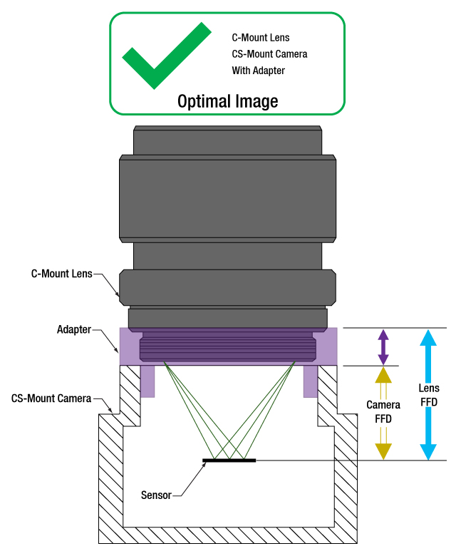
Click to Enlarge
Figure 4: An adapter with the proper thickness moves the C-mount lens away from the CS-mount camera's sensor by an optimal amount, which is indicated by the length of the purple arrow. This allows the lens to focus light on the camera's sensor, despite the difference in FFD.
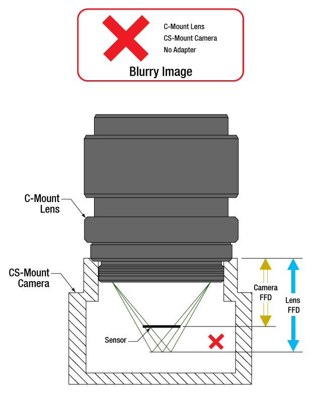
Click to Enlarge
Figure 3: A C-mount lens and a CS-mount camera are not directly compatible, since their flange focal distances, indicated by the blue and yellow arrows, respectively, are different. This arrangement will result in blurry images, since the light will not focus on the camera's sensor.
Date of Last Edit: July 21, 2020
Do Thorlabs' scientific cameras need an adapter?
Click to Enlarge
Figure 6: An adapter can be used to optimally position a C-mount lens on a camera whose flange focal distance is less than 17.526 mm. This sketch is based on a Zelux camera and its SM1A10Z adapter.
Click to Enlarge
Figure 7: An adapter can be used to optimally position a CS-mount lens on a camera whose flange focal distance is less than 12.526 mm. This sketch is based on a Zelux camera and its SM1A10 adapter.
All Kiralux™ and Quantalux® scientific cameras are factory set to accept C-mount lenses. When the attached C-mount adapters are removed from the passively cooled cameras, the SM1 (1.035"-40) internal threads in their flanges can be used. The Zelux® scientific cameras also have SM1 internal threads in their mounting flanges, as well as the option to use a C-mount or CS-mount adapter.
The SM1 threads integrated into the camera housings are intended to facilitate the use of lens assemblies created from Thorlabs components. Adapters can also be used to convert from the camera's C-mount configurations. When designing an application-specific lens assembly or considering the use of an adapter not specifically designed for the camera, it is important to ensure that the flange focal distances (FFD) of the camera and lens match, as well as that the camera's sensor size accommodates the desired field of view (FOV).
Made for Each Other: Cameras and Their Adapters
Fixed adapters are available to configure the Zelux cameras to meet C-mount and CS-mount standards (Figures 6 and 7). These adapters, as well as the adjustable C-mount adapters attached to the passively cooled Kiralux and Quantalux cameras, were designed specifically for use with their respective cameras.
While any adapter converting from SM1 to 1.000"-32 threads makes it possible to attach a C-mount or CS-mount lens to one of these cameras, not every thread adapter aligns the lens' focal plane with a specific camera's sensor plane. In some cases, no adapter can align these planes. For example, of these scientific cameras, only the Zelux can be configured for CS-mount lenses.
The position of the lens' focal plane is determined by a combination of the lens' FFD, which is measured in air, and any refractive elements between the lens and the camera's sensor. When light focused by the lens passes through a refractive element, instead of just travelling through air, the physical focal plane is shifted to longer distances by an amount that can be calculated. The adapter must add enough separation to compensate for both the camera's FFD, when it is too short, and the focal shift caused by any windows or filters inserted between the lens and sensor.
Flexiblity and Quick Fixes: Adjustable C-Mount Adapter
Passively cooled Kiralux and Quantalux cameras consist of a camera with SM1 internal threads, a window or filter covering the sensor and secured by a retaining ring, and an adjustable C-mount adapter.
A benefit of the adjustable C-mount adapter is that it can tune the spacing between the lens and camera over a 1.8 mm range, when the window / filter and retaining ring are in place. Changing the spacing can compensate for different effects that otherwise misalign the camera's sensor plane and the lens' focal plane. These effects include material expansion and contraction due to temperature changes, positioning errors from tolerance stacking, and focal shifts caused by a substitute window or filter with a different thickness or refractive index.
Adjusting the camera's adapter may be necessary to obtain sharp images of objects at infinity. When an object is at infinity, the incoming rays are parallel, and location of the focus defines the FFD of the lens. Since the actual FFDs of lenses and cameras may not match their intended FFDs, the focal plane for objects at infinity may be shifted from the sensor plane, resulting in a blurry image.
If it is impossible to get a sharp image of objects at infinity, despite tuning the lens focus, try adjusting the camera's adapter. This can compensate for shifts due to tolerance and environmental effects and bring the image into focus.
Date of Last Edit: Aug. 2, 2020
Why can the FFD be smaller than the distance separating the camera's flange and sensor?
Flange focal distance (FFD) values for cameras and lenses assume only air fills the space between the lens and the camera's sensor plane. If windows and / or filters are inserted between the lens and camera sensor, it may be necessary to increase the distance separating the camera's flange and sensor planes to a value beyond the specified FFD. A span equal to the FFD may be too short, because refraction through windows and filters bends the light's path and shifts the focal plane farther away.
If making changes to the optics between the lens and camera sensor, the resulting focal plane shift should be calculated to determine whether the separation between lens and camera should be adjusted to maintain good alignment. Note that good alignment is necessary for, but cannot guarantee, an in-focus image, since new optics may introduce aberrations and other effects resulting in unacceptable image quality.
Click to Enlarge
Figure 9: Refraction causes the ray's angle with the optical axis to be shallower in the medium than in air (θm vs. θo ), due to the differences in refractive indices (nm vs. no ). After travelling a distance d in the medium, the ray is only hm closer to the axis. Due to this, the ray intersects the axis Δf beyond the f point.
Click to Enlarge
Figure 8: A ray travelling through air intersects the optical axis at point f. The ray is ho closer to the axis after it travels across distance d. The refractive index of the air is no .
| Example of Calculating Focal Shift | |||
|---|---|---|---|
| Known Information | |||
| C-Mount FFD | f | 17.526 mm | |
| Total Glass Thickness | d | ~1.6 mm | |
| Refractive Index of Air | no | 1 | |
| Refractive Index of Glass | nm | 1.5 | |
| Lens f-Number | f / N | f / 1.4 | |
| Parameter to Calculate |
Exact Equations | Paraxial Approximation |
|
| θo | 20° | ||
| ho | 0.57 mm | --- | |
| θm | 13° | --- | |
| hm | 0.37 mm | --- | |
| Δf | 0.57 mm | 0.53 mm | |
| f + Δf | 18.1 mm | 18.1 mm | |
| Equations for Calculating the Focal Shift (Δf ) | ||
|---|---|---|
| Angle of Ray in Air, from Lens f-Number ( f / N ) |  |
|
| Change in Distance to Axis, Travelling through Air (Figure 8) |  |
|
| Angle of Ray to Axis, in the Medium (Figure 9) |
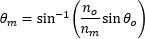 |
|
| Change in Distance to Axis, Travelling through Optic (Figure 9) |  |
|
| Focal Shift Caused by Refraction through Medium (Figure 9) | Exact Calculation |
 |
| Paraxial Approximation |
 |
|
Click to Enlarge
Figure 11: Tolerance and / or temperature effects may result in the lens and camera having different FFDs. If the FFD of the lens is shorter, images of objects at infinity will be excluded from the focal range. Since the system cannot focus on them, they will be blurry.
Click to Enlarge
Figure 10: When their flange focal distances (FFD) are the same, the camera's sensor plane and the lens' focal plane are perfectly aligned. Images of objects at infinity coincide with one limit of the system's focal range.
A Case of the Bends: Focal Shift Due to Refraction
While travelling through a solid medium, a ray's path is straight (Figure 8). Its angle
When an optic with plane-parallel sides and a higher refractive index
While travelling through the optic, the ray approaches the optical axis at a slower rate than a ray travelling the same distance in air. After exiting the optic, the ray's angle with the axis is again θo , the same as a ray that did not pass through the optic. However, the ray exits the optic farther away from the axis than if it had never passed through it. Since the ray refracted by the optic is farther away, it crosses the axis at a point shifted Δf beyond the other ray's crossing. Increasing the optic's thickness widens the separation between the two rays, which increases Δf.
To Infinity and Beyond
It is important to many applications that the camera system be capable of capturing high-quality images of objects at infinity. Rays from these objects are parallel and focused to a point closer to the lens than rays from closer objects (Figure 10). The FFDs of cameras and lenses are defined so the focal point of rays from infinitely distant objects will align with the camera's sensor plane. When a lens has an adjustable focal range, objects at infinity are in focus at one end of the range and closer objects are in focus at the other.
Different effects, including temperature changes and tolerance stacking, can result in the lens and / or camera not exactly meeting the FFD specification. When the lens' actual FFD is shorter than the camera's, the camera system can no longer obtain sharp images of objects at infinity (Figure 11). This offset can also result if an optic is removed from between the lens and camera sensor.
An approach some lenses use to compensate for this is to allow the user to vary the lens focus to points "beyond" infinity. This does not refer to a physical distance, it just allows the lens to push its focal plane farther away. Thorlabs' Kiralux™ and Quantalux® cameras include adjustable C-mount adapters to allow the spacing to be tuned as needed.
If the lens' FFD is larger than the camera's, images of objects at infinity fall within the system's focal range, but some closer objects that should be within this range will be excluded. This situation can be caused by inserting optics between the lens and camera sensor. If objects at infinity can still be imaged, this can often be acceptable.
Not Just Theory: Camera Design Example
The C-mount, hermetically sealed, and TE-cooled Quantalux camera has a fixed 18.1 mm spacing between its flange surface and sensor plane. However, the FFD (f ) for C-mount camera systems is 17.526 mm. The camera's need for greater spacing becomes apparent when the focal shift due to the window soldered into the hermetic cover and the glass covering the sensor are taken into account. The results recorded in the table beneath Figure 9 show that both exact and paraxial equations return a required total spacing of 18.1 mm.
Date of Last Edit: July 31, 2020
How can a manual translation stage be motorized?
The movement of Thorlabs' manual translation stages is driven by a micrometer or other adjuster, which can be replaced with a motorized actuator that has a compatible travel range and barrel diameter. Before making the substitution, it is important to fully retract the installed adjuster to protect the stage from the mechanical shock of a sudden release of spring energy.
Video Clip 1: It is important to completely retract the installed micrometer or other adjuster as the first step. If the adjuster is extended when it is released from the stage, the top plate of the stage will be propelled backwards into a hard stop. The mechanical shock may damage the stage.
Video Clip 3: After the micrometer on the XR25P stage is completely retracted, the locking cap screw on the stage's barrel clamp can be loosened with a 5/64" (2 mm) hex key and the adjuster removed. The barrel of the motorized actuator, which is the DC-servo-motor-driven Z825B in this example, is then inserted and the locking setscrew is tightened until snug.
Video Clip 2: After the adjustment screw on the MT1B stage is completely retracted, the locking cap screw on the stage's barrel clamp can be loosened with a 3/32" hex key and the adjuster removed. The barrel of the motorized actuator, which is the stepper-motor-driven ZFS13B in this example, is then inserted and the locking setscrew is tightened until snug.
Check Barrel Diameter and Travel Range Compatibility
These stages secure the actuator using a barrel clamp, which makes it necessary to match the actuator's barrel diameter to the clamp's specifications. Both stages chosen for this demonstration accept actuators with a 3/8" (9.5 mm) diameter barrel.
The travel range of the actuator must not exceed that of the stage. An actuator with a larger travel range can potentially force the stage to extend beyond its limit, which may damage both the stage and the actuator's motor. An actuator with a shorter travel range will cause no mechanical harm to itself or the stage, but the stage's travel range will be reduced. The MT1B and XR25P linear translation stages included in this demonstration have travel ranges of 0.5" and 1" (13 mm and 25 mm), respectively.
Retract the Adjuster to Avoid Damaging the Stage
Fully retracting the installed adjuster, before doing anything else, avoids a significant cause of damage to these stages. When the adjuster is fully retracted, the top plate is positioned as far backwards as possible to relieve the spring tension. Ideally, the tip of the adjuster would no longer be in contact with the stage.
An extended position is dangerous due to the force exerted by the stage's internal springs. The spring force keeps the top plate, or moving world, in contact with the tip of the adjuster (Clip 1). If the adjuster is extended when it is released from the stage, the spring force on the top plate will propel it backwards into a hard stop. The mechanical shock of this collision can be severe and potentially misalign the stage's components, affect the ball bearings, and introduce angular deviations to the stage's travel.
Make the Replacement
With the installed adjuster completely retracted, the locking cap screw in the barrel clamp of the MT1B or XR25P stage can be loosened using a 3/32" or 5/64" (2 mm) hex key, respectively. This will release the holding force on the barrel of the adjuster, so that it can be removed (Clips 2 and 3).
Insert the barrel of the motorized actuator and tighten the locking cap screw until it is snug, but not too tight. The spring load on the top plate should not be able to push the actuator out of the barrel clamp, but the locking screw should not be so tight that it deforms the barrel, which could affect the linearity of the actuator.
Want additional Insights on translation stages?
Watch the full video.
Date of Last Edit: Nov. 11, 2023
Recording Position from Digital Micrometers
Click to Enlarge
Figure 2: The SBC-COMM package shown above can be used to log data position data displayed by the DM713 digital micrometer.

Click to Enlarge
Figure 1: The DM713 digital micrometer (right) is included with and used to adjust the retardance provided by the SBC-VIS Soleil-Babinet compensator (left).
Digital micrometers, such as the DM713, are handy for moving a piece of optomech a specific distance. For example, a user might want to increment a translation stage holding a sample in front of an objective lens in order to focus the light to equally spaced points within the sample.
However, there are also times where the user might want to record the position of an event. One example could be making a distance measurement where the micrometer is set to a starting position, zeroed, and then translated the desired amount to display the distance.
Using the DM713 alone creates an extra step where the user has to read and record the display, which can be tedious in a dark lab where the display is not visible. One solution is to use Thorlabs' SBC-COMM, which includes an RS-232 interfacing cable. Thorlabs has created software application notes that walk the user through creating Visual C#® and LabVIEW® programs to continuously measure distances with the DM713.
Another solution is to purchase the Mitutoyo® 05CZA662 SPC cable and IT-016U USB input tool that provide a push button and USB interfacing cable. With this device the user can open any text entry software package, press the single push button, and the device acts like a keyboard to enter the number into the software.
Date of Last Edit: Dec. 4, 2019
Insights into Off-Axis Parabolic Mirrors
Scroll down or click on one of the following links to read about the unique properties of off-axis parabolic (OAP) mirrors and how to take advantage of them.
- Why use a parabolic mirror instead of a spherical mirror?
- Benefit of an Off-Axis Parabolic Mirror
- The Off-Axis Angle of an OAP Mirror
- Focus Collimated Light / Collimate Light from a Point Source Using an OAP Mirror
- Locating the Optical and Focal Axes of an OAP Mirror
- Paired OAP Mirrors Can Relay an Image and Make the Beam Accessible
- Mounting and Aligning an OAP Mirror
- Directionality of OAP-Mirror-Based Reflective Collimators
Why use a parabolic mirror instead of a spherical mirror?
Click to Enlarge
Figure 2: Spherical mirrors do not reflect all rays in a collimated beam through a single point. A selection of intersections in the focal volume are indicated by black dots.
Click to Enlarge
Figure 1: Parabolic mirrors have a single focal point for all rays in a collimated beam.
Parabolic mirrors perform better than spherical mirrors when collimating light emitted by a point source or focusing a collimated beam.
Focusing Collimated Light
Parabolic mirrors (Figure 1) focus all rays in an incoming, collimated light beam to a diffraction-limited spot. In contrast, concave spherical mirrors (Figure 2) concentrate incoming collimated light into a volume larger than a diffraction-limited spot. The size of the spherical mirror's focal volume can be reduced by decreasing the diameter of the incoming collimated beam.
Collimating Light from a Point Source
A point source emits light in all directions. When this highly divergent light source is placed at the focal point of a parabolic mirror, the output beam is highly collimated. If the point source were ideal, all reflected rays would be perfectly parallel with one another.
When a point source is placed within a spherical mirror's focal volume, the output beam is not as well collimated as the beam provided by a parabolic mirror. Different rays from the point source are not perfectly parallel after reflection from the spherical mirror, but two reflected rays will be more nearly parallel when they reflect from more closely spaced points on the spherical mirror's surface. Consequently, the quality of the collimated beam can be improved by reducing the area of the reflective surface. This is equivalent to limiting the angular range over which the source in the focal volume emits light.
Choosing Between Parabolic and Spherical Mirrors
A parabolic mirror is not always the better choice. Beam diameter, cost constraints, space limitations, and performance requirements of an application all influence selection. Beam diameter is a factor, since the performance of these two mirrors is more similar when the beam diameter is smaller. Parabolic mirrors are more expensive, since their reflective profiles are more difficult to fabricate. Parabolic mirrors are also typically larger. Improved performance may or may not be more important than the difference in cost and physical size.
Date of Last Edit: Dec. 4, 2019
Benefit of an Off-Axis Parabolic Mirror
Click to Enlarge
Figure 4: An off-axis parabolic mirror can be thought of as a section of the larger parabolic shape. Both have the same focal point, but it is more accessible in the case of an OAP mirror.
Click to Enlarge
Figure 3: The focal point of an on-axis parabolic mirror is close to the reflective surface, and typically surrounded by the reflective surface, which makes the focal point difficult to access.
Both symmetric parabolic and off-axis parabolic (OAP) mirrors have a single focal point. The benefit of an OAP mirror is that its focal point is accessible, unlike that of a symmetric parabolic mirror.
The single focal point is a primary benefit parabolic mirrors and is useful for a range of purposes, including imaging and manufacturing applications that require focusing laser light to a diffraction limited spot.
There are a few negatives associated using with using conventional parabolic mirrors, which are symmetric around the focal point (Figure 3). One is that the sides of the mirror generally obstruct access to the focus. Another is that when the mirror is used to collimate a divergent light source, the housing of the light source blocks a portion of the collimated beam. In particular, light emitted at small angles with respect to the optical axis of the mirror is typically obstructed.
An off-axis parabolic (OAP) mirror (Figure 4) is one solution to this problem. The reflective surface of this mirror is parabolic in shape, but it is not symmetric around the focal point. The reflective surface of the OAP corresponds to a section of the parent parabola that is shifted away from the focal point. The section chosen depends on the desired angle and / or distance between the focal point and the center of the mirror.
Date of Last Edit: Dec. 4, 2019
The Off-Axis Angle of an OAP Mirror

Click to Enlarge
Figure 6: One section of the parent parabola provides a 90° off-axis angle.
Click to Enlarge
Figure 5: It is common to measure the width of the parabola with respect to a line that passes through the focus and is perpendicular to the axis.
Click to Enlarge
Figure 8: Decreasing the width of the parabola increases the off-axis angle. For example, compare this illustration with Figure 5.
Click to Enlarge
Figure 7: Choosing a section closer to the axis of the parabola results in a smaller off-axis angle.
The off-axis angle (θ ) of an OAP mirror is measured between the mirror's optical and focal axes. The angle depends on the segment of the parent parabola used for the OAP mirror, as well as the width (Figure 6) of the parent parabola. The OAP mirror in Figure 5 has a 90° angle.
Proximity of Parabolic Segment and Focal Point
Choosing a segment of the parent parabola closer to the focal point reduces the off-axis angle. The mirror in Figure 7 has a smaller angle than the one in Figure 5, but the only difference between them is that the section of the parabola selected for the OAP mirror in Figure 7 is closer to the focal point.
The location of the parabolic segment also controls the focal length. Choosing a parabolic segment closer to the focal point results in a shorter distance between the center of the mirror and the focal point.
Width of the Parent Parabola
Increasing the width of the parent parabola decreases the off-axis angle. This inverse relationship is illustrated by Figures 7 and 8. The width of the parabola is larger in Figure 7, and this is also the mirror with a smaller angle.
The width of the parent parabola also affects the focal length. The wider the parabola, the longer the focal length.
Available Off-Axis Angles
OAP mirrors are often designed to have a 90° off-axis angle, but OAP mirrors with angles less than 90° are also common.
Date of Last Edit: Dec. 4, 2019
Focus Collimated Light / Collimate Light from a Point Source Using an OAP Mirror
Click to Enlarge
Figure 9: The focal and optical axes of an OAP mirror do not coincide and are not parallel.
Click to Enlarge
Figure 11: When the collimated beam is not directed along the mirror's optical axis, the mirror does not provide a diffraction-limited spot. Instead, the focal region is spread out.
Click to Enlarge
Figure 10: When the collimated beam is parallel to the optical axis of a parabolic or OAP mirror, the light focuses to a diffraction-limited spot.
Parabolic and off-axis parabolic (OAP) mirrors will only provide the expected well-collimated beam or diffraction-limited focal spot when the correct beam type is incident along the proper axis. This due to the parabolic shape of these mirrors' reflective surfaces, which are not symmetric around their focal points.
Parabolic vs. Off-Axis Parabolic Mirrors
The reflective surface of an OAP mirror is a section of the parent parabola that is not centered on the parent's optical axis (Figure 9). A conventional parabolic mirror is illustrated in Figure 10.
The optical axis of an OAP mirror is parallel to, but displaced from the optical axis of the parent parabola. The focal point of the OAP mirror coincides with that of the parent parabola.
The focal axis of the OAP mirror passes through the focal point and the center of the OAP mirror. The focal and optical axes of an OAP mirror are not parallel. In contrast, these axes coincide for parabolic mirrors whose reflective surfaces are centered on optical axis of the parent parabola.
Focus Collimated Light
If a parabolic or OAP mirror is being used to focus a beam of collimated light to a diffraction-limited point, the light must be directed along the mirror's optical axis (Figures 9 and 10).
Collimated light that is not directed parallel to the optical axis will not focus to a unique point (Figure 11).
Thorlabs recommends against directing collimated light along the focal axis of OAP mirrors, or along any direction that is not parallel to the optical axis, since the light will not focus to a diffraction-limited spot.
Collimate Light from a Point Source
To obtain highly collimated light from a point source, the point source should be located at the mirror's focal point.
Light from a point source will be poorly collimated if the point source is placed along the OAP mirror's optical axis, or anywhere else that is not the focal point.
An OAP mirror can also be used to collimate a spherical wave, if its origin coincides with the focal point of the mirror.
Date of Last Edit: Dec. 4, 2019
Locating the Optical and Focal Axes of an OAP Mirror
Click to Enlarge
Figure 13: The orientation of the optical axis can be found by noting it is perpendicular to the base of the mirror's substrate. The location of the focal point can be estimated by considering collimated light rays that are directed parallel to the optical axis. These rays reflect symmetrically around the local surface normals and pass through the mirror's focal point.
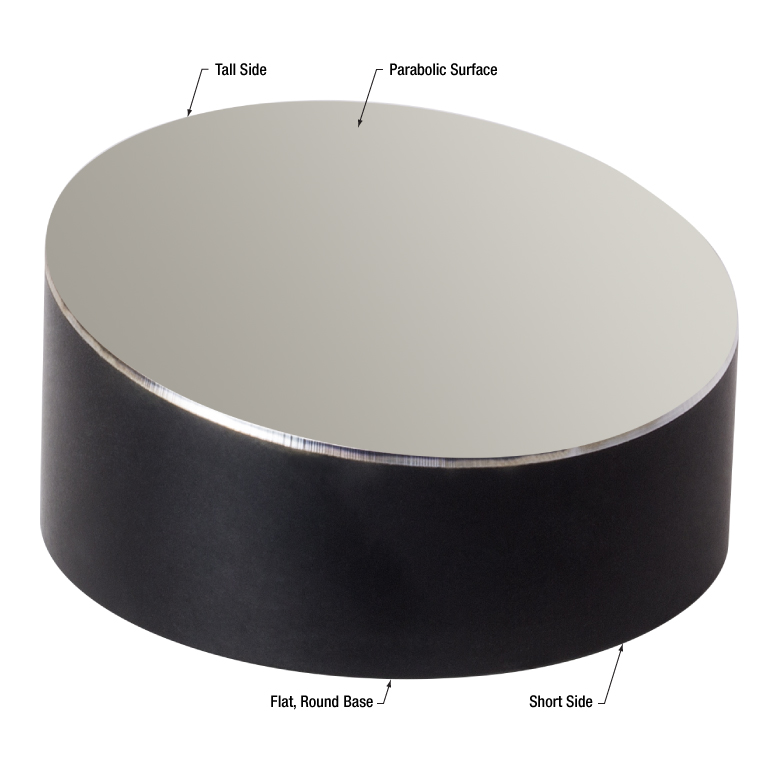
Click to Enlarge
Figure 12: OAP mirrors have a flat, round base and a side that varies in height around the circumference. The planar base is normal to the mirror's optical axis. Shown above is the MPD2151-P01.
When working with off-axis parabolic (OAP) mirrors, it can be challenging to identify the optical and focal axes. This is particularly true when the parabolic curvature of the surface is hard to see (Figure 12).
The physical characteristics and dimensions of the mirror's substrate can provide a useful guide when positioning and aligning the mirror.
The mirror's substrate has a flat, round base. The optical axis is oriented normal to this planar base. Therefore, collimated light should be directed normal to the surface of the base.
The substrate has a tall side and a short side, and the reflective surface is sloped between them. The surface normal at different points across the reflector can be roughly estimated by visually examining the surface (Figure 13).
The location of the focal point can be estimated by considering a ray of collimated light, parallel to the optical axis, that reflects from the surface of the mirror. The incident ray reflects symmetrically about the surface normal. The reflected ray will pass through the focal point. By mentally tracing two rays from positions close to the tall and short sides of the mirror, respectively, it should be possible to estimate the location of the focal point.
Mounting and Alignment Features on Thorlabs' OAP Mirrors
Thorlabs' OAP mirrors have an alignment hole and three tapped mounting holes machined into the bottom surface of their bases. The pattern of tapped holes matches the vertices of an equilateral triangle, and the position of the smooth-bore alignment hole indicates the short side of the OAP mirror. The tapped holes are designed to secure the mirror to mounting adapters or mounting platforms.
Date of Last Edit: Dec. 4, 2019
Paired OAP Mirrors Can Relay an Image and Make the Beam Accessible
Click to Enlarge
Figure 15: A pair of OAP mirrors can be used to couple light out of one fiber and into another. This provides access to the beam when it is necessary to insert bulk optics into the optical path. Due to the small dimension of the fiber core, light emitted from the fiber end face is similar to a point source.
Click to Enlarge
Figure 14: A pair of OAP mirrors can be used in imaging applications, and/or to relay a beam across a distance.
Relay an Image
A pair of OAP mirrors can act as a relay, as illustrated in Figures 14 and 15, since the light traveling between the mirrors is collimated. Since OAP mirrors are only designed to collimate light from a focal point, or focus collimated light, two mirrors should be used when neither the source nor the image light is collimated (finite conjugate imaging).
The dual OAP configuration facilitates the process of adjusting the distance between mirrors. The leg of collimated light is also convenient for inserting filters and other optical elements into the beam. Another benefit is that distance between the two mirrors can be adjusted to move the focal point across the source and/or target planes without disturbing the alignment of the system.
Provide Access to the Beam in a Fiber Network
A pair of OAP mirrors can be used to create a free-space leg in an optical fiber system, which is one way to provide access to the light beam. The illustration in Figure 15 shows an example of this configuration, which can be useful when filters or other bulk optics need to be inserted into the beam path. The length of the free-space leg can be adjusted without disturbing alignment.
When setting up this system, the fibers' end faces must be aligned so that their cores coincide with the source and target focal points, respectively. The collimated beam paths of both mirrors should be co-linear and completely overlapping.
This configuration is the basis for fiber optic filter / attenuator mounts.
Date of Last Edit: Dec. 4, 2019
Mounting and Aligning an OAP Mirror
Click to Enlarge
Figure 17: When using an OAP mirror to collimate a point source, a shear plate interferometer placed in the output beam can facilitate the alignment process.
Click to Enlarge
Figure 16: The shape of the OAP mirror's reflective profile matches a section of the parent parabola that is not centered on the focal point. Due to this, the OAP's reflective surface is not rotationally symmetric. When mounting the mirror, care should be taken to ensure the mirror does not rotate around its optical axis.
OAP mirrors are not rotationally symmetric. This is a consequence of their reflective surfaces being taken from sections of the parent parabola curve located away from the focal point (Figure 16). Due the asymmetry of the reflector, when an OAP mirror rotates, the position of its focal point also rotates. Since this could negatively impact the performance of an optical system, the mirror should be fixed so that the reflective surface cannot rotate around its optical axis.
The optical performance of the mirror is also sensitive to alignment drift with respect to the other five degrees of freedom. One way to protect against alignment drift is to use a fixed, rather than a kinematic, mount.
Using a shear plate interferometer can be helpful when aligning an OAP mirror to an input point source. The shear plate interferometer should intercept the output beam (Figure 17), to assess its collimation quality. Alignment is optimized when the quality of the collimated beam is optimized.
Date of Last Edit: Dec. 4, 2019
Directionality of OAP-Mirror-Based Reflective Collimators
The two ports on Thorlabs' reflective collimators are not interchangeable. One port accepts an optical fiber connector and requires the highly divergent light of a point source. The other port is designed solely for collimated, free-space light (Figure 18).
Click to Enlarge
Figure 19: The reflective element of the collimator is an off-axis parabolic mirror. The mirror's substrate is highlighed in red. The shape of the reflective surface is a segment of the parabolic curve displaced from the vertex. The focal points of the parent parabola and the OAP mirror coincide.
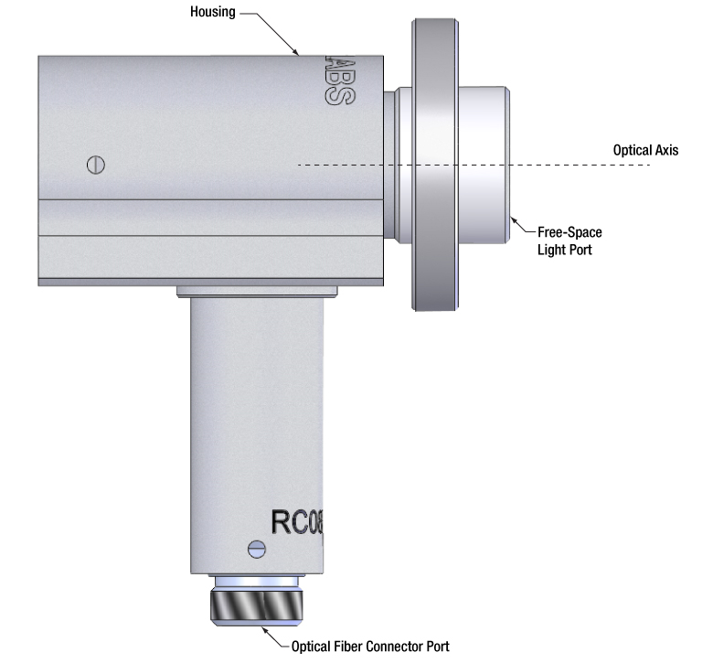
Click to Enlarge
Figure 18: Thorlabs offers reflective collimators that include a port for an optical fiber connector and a port for free space, collimated light that propagates parallel to the optical axis.
Free Space Port
Light input to this port should be collimated and directed parallel to the optical axis. Diverging light from a fiber end face, a laser diode, or other source should not be input. This light would not be collimated at the fiber connector port or coupled into the fiber connected to the fiber port.
Optical Fiber Connector Port
This port aligns the fiber's end face with the focal point of the mirror. Since the fiber's end face approximates a point source placed at the focal point, a collimated beam is output from the free-space port. The alignment of the fiber end face with the focal point is also the reason that all light input to the free-space light port should be collimated and directed parallel to the optical axis.
Source of Directionality
The collimator's directionality is a consequence of using a non-rotationally symmetric, off-axis parabolic (OAP) mirror as the reflective element (Figure 19). The cut-away view illustrates that the fiber's end face is positioned at the focal point of the parent parabola, which is also the focal point of the OAP mirror.
Date of Last Edit: Dec. 4, 2019
Insights into Optical Isolators and the Faraday Effect
Scroll down or click on the following link to read about an approach used to measure the strength of the Faraday Effect.
- How can the strength of a material's Faraday effect be measured?
- What is needed to determine the direction and magnitude of the Faraday rotation angle?
How can the strength of a material's Faraday effect be measured?
Since the Faraday effect causes the polarization state of light to rotate as it propagates through a material in the presence of a magnetic field, one approach to determining the effect's strength in a material is to input linearly polarized light, apply a strong magnetic field through the material, and observe the induced change in the orientation of the output polarization state. It is not necessary to directly measure the output polarization state to determine the change in its orientation. Instead, the output light can be analyzed by measuring the optical power transmitted through a rotating linear polarizer. The measured power oscillates with a phase dependent on the orientation of the linear polarization state incident on the rotating polarizer. This was demonstrated using a CdMgTe crystal. Measurements of light output from the crystal were used to calculate its Verdet constant, which characterizes the strength of a material's Faraday effect.
Click to Enlarge
Figure 1: Faraday effect measurements can be made with the sample placed between a linearly polarized light source and a polarization-sensitive detection system. The CdMgTe crystal was approximately a third of the length of the annular magnet's bore, and the plastic sample holder was used to position and immobilize the crystal at the center of the bore. In the detection system, the optical power sensor was placed as close as possible to the output side of the linear polarizer, which was installed in an indexed rotation mount. An advantage of this setup is that it requires minimal alignment.
Click to Enlarge
Figure 3: Optical power measurements were made while rotating the detection polarizer's transmission axis in 2° increments. Data were acquired with the magnet out of (triangles) and in (squares) the setup. Malus' law (solid lines) was used to model a to fit each curve. The phase shift
Click to Enlarge
Figure 2: The crystal under test was placed in the bore of the annular magnet (left). The 2.2 mm long crystal was positioned in the center of the 6.35 mm long bore, where the magnetic field was strongest, most uniform, and directed along the N-S axis (right).
| Curve Fit to Data Acquired Without Magnet |
Curve Fit to Data Acquired With Magnet |
Faraday Rotation (Δθ ) |
 |
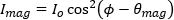 |
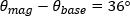 |
Faraday Rotation
The rotation of the polarization state due to the Faraday effect is called the Faraday rotation, which is directly proportional to both the magnetic field strength (B ) in the material and the physical distance (L ) the light propagates through the material in the presence of the field. The proportionality constant is called the Verdet constant (V ).
This intrinsic material parameter, which is wavelength and temperature dependent, characterizes the strength of the material's Faraday effect. When the Verdet constant is known, the Faraday rotation (Δθ ),

due to different magnetic field strengths and material lengths can be calculated. One approach to obtaining the Verdet constant is to measure the Faraday rotation for a specific material length and a known magnetic field strength.
Faraday Effect Measurement
Using this approach, and the setup illustrated in Figure 1, the strength of a CdMgTe crystal's Faraday effect was measured.
The linearly polarized light source consisted of a collimated fiber-coupled laser whose 785 nm emission was transmitted through a fixed linear polarizer.
An annular super magnet was used in order to provide a magnetic field strong enough to induce a measurable Faraday rotation. The crystal was mounted in the center of the magnet's bore, as that is where the magnetic field is the strongest (Figure 2).
The light output from the crystal was transmitted through a second linear polarizer, which was secured in an indexed rotation mount, and to a power sensor. The power sensor was positioned as close as possible to the output side of the linear polarizer.
Two measurement sets were acquired, one with, and the other without, the magnet in the setup. Each data set (Figure 3) recorded average power measurements taken at 2° increments of the second linear polarizer's transmission axis angle. The curves oscillate with the same period but are phase shifted
Calculate the Verdet Constant
The phase shift between the two curves plotted in Figure 3 is related to the Faraday rotation. As is described in a separate Insight, it is in general necessary to add a factor of  to the phase shift to obtain the Faraday rotation. In this case, that factor is equal to zero and the phase shift equals the Faraday rotation.
The phase shift can be determined after each data curve is fit using Malus' law,
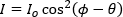 ,
,
in which Io is the intensity of the incident light and  is the angle of the second linear polarizer's transmission axis. The fit parameter (θ ) is a constant that was optimized individually (θbase and θmag , respectively, in the table) for each data set. The difference in the two fit parameters is the Faraday rotation (36°). Using this Faraday rotation value, the Verdet constant can be calculated,
,
in which Io is the intensity of the incident light and is the angle of the second linear polarizer's transmission axis. The fit parameter (θ ) is a constant that was optimized individually (θbase and θmag , respectively, in the table) for each data set. The difference in the two fit parameters is the Faraday rotation (36°). Using this Faraday rotation value, the Verdet constant can be calculated,

The magnetic field strength (B ) was 5800 Gauss at the center of the magnet's bore, the crystal's length (L ) was 0.22 cm, and the Faraday rotation angle
Content contributed by and based on work performed by Zoya Shafique.
Date of Last Edit: May 20, 2021
What is needed to determine the direction and magnitude of the Faraday rotation angle?
An approach for determining the direction and magnitude of the Faraday rotation angle uses both linearly polarized input light and a magnetic field whose applied strength can be adjusted. Faraday rotation is a consequence of the Faraday effect, which causes the polarization orientation of linearly polarized light to rotate as it propagates through a material in the presence of a magnetic field. The Faraday rotation angle can be characterized by analyzing magnetic-field dependent measurements of the polarization orientation of the light output from the material. The angular difference between the polarization orientations of the light input to and output from the material is measured for each magnetic field strength value. This set of angular difference values can then be used to determine the Faraday rotation angle for a particular magnetic field strength, as is demonstrated using the example of a fixed-length CdMgTe crystal.
Click to Enlarge
Figure 1: The Faraday effect causes linearly polarized light to rotate around the optical axis. The direction of rotation and the number of rotations depends on the applied magnetic field, the propagation direction of the light, and material properties. The direction and magnitude of the Faraday rotation (Δθ ) cannot be determined by measuring the angular difference ( ) between polarization orientations of the light input to and output from the material, since these angles are mapped to an angular range between 0 and .
Click to Enlarge
Figure 3: The magnetic field through the bore of the annular super magnet used in this work was calculated. The points labeled on this plot are also labeled in Figure 2. Point A corresponds to the center of the bore, and the field is zero at point C. The magnetic field strength is positive when it is directed towards the magnet's south pole.
Click to Enlarge
Figure 2: The annular super magnet used in this work is illustrated. The calculated magnetic field along the N-S axis is modeled in Figure 3. The magnetic field at points labeled in this image are indicated on the plot. At point C, the field lines cancel each other. The direction of the field also reverses at this point.
Click to Enlarge
Figure 4: Plotting the calculated angles (Δθtrial ) and the measured angles () together is one way to visualize their relationship. The value of measured for an applied magnetic field value of 5800 Gauss was used to calculate a constant (Vtrial ), which was then used to calculate Δθtrial as described in the table. Since the Δθtrial and measured values are in good agreement, the measured angles equal the Faraday rotation angles.
| Trial Verdet Constant Calculation (Vtrial ) |
 |
| Trial Faraday Rotation Calculation (Δθtrial ) |
 |
Faraday Rotation Angle
The direction of the Faraday rotation around the optical axis depends on the orientation of the magnetic field
also depends on the propagation distance
Measured Angle
A technique that compares the polarization orientations of the linearly polarized light input to, and output from, the material provides an angular value (). However, this approach automatically maps each angle to the range between 0 and , and neither the rotation direction, or the number of rotations the linearly polarized light made around the optical axis (Figure 1) is known.
Varying the Magnetic Field Strength
If values of are measured for different applied magnetic fields, the Faraday rotation angle for a particular applied field can be determined. The applied field can be changed by moving the material to different positions within a static, but spatially varying, magnetic field.
For example, the magnetic field strength within the bore of an annular super magnet varies with distance along the N-S axis, while the field's direction remains parallel to the axis (Figures 2 and 3). The plot of the magnetic field in Figure 3 was calculated based on a model of the annular super magnet.
The magnetic field strength can be varied, without changing the field's direction, by translating the sample along the N-S axis. In this work, the sample was moved to specific points along this axis, and the position was measured with respect to the center of the magnet's bore.
Characterizing the Faraday Rotation
A convenient starting point for characterizing the Faraday rotation angle is to assume values of , measured for different applied magnetic field values, have the same magnitude as the corresponding Faraday rotation angles. The next step is to test this assumption.
This procedure was followed to determine the direction and magnitude of the Faraday rotation angle when a magnetic field is applied to a 0.22 cm long CdMgTe crystal. An annular super magnet provided the magnetic field, and values of were calculated for measurements made with the crystal placed at various points along the N-S axis. The crystal was moved between the points A and C labeled in Figure 2. Within this range, the light propagates along the direction of the magnetic field. After point C, the magnetic field direction reverses.
A trial Verdet constant (Vtrial , table) was calculated using the value of (2160 arcmin) and the corresponding magnetic field strength (5800 Gauss). Then trial Faraday rotation angles (Δθtrial , table) were calculated using Vtrial . Since the measured and the modeled data are in good agreement (Figure 4), the measured values of are equal to the Faraday rotation angles. The differences between the calculated and measured angles are attributed mostly to differences between the modeled and actual magnetic fields, although measurement error may also contribute. The data plotted in Figure 4 indicate the sign of the calculated Verdet constant is positive, as well as establish that can be used in the equation to calculate an accurate value of the Verdet constant.
When the two sets of angular data do not agree, the actual Faraday rotation angle is the sum of the measured angle value and a factor of . A special case is when the measured angles and the calculated trial Faraday rotation angles both have the same magnitude, but their signs are opposite. The two angles then differ by and the actual and trial Verdet constants have opposite signs.
Content contributed by and based on work performed by Zoya Shafique.
Date of Last Edit: May 20, 2021
How does wavelength affect rise time?
Click to Enlarge
Figure 2: Typical absorption coefficients and penetration depths for silicon, germanium, and indium gallium arsenide (In0.53Ga0.47As) are plotted. The penetration depth is the reciprocal of the absorption coefficient.
Click to Enlarge
Figure 1: Different wavelengths of light have different average penetration depths into the PN-junction based detector. The penetration depth is related to the wavelength-dependent absorption coefficient (Figure 2).
When light is incident upon a photodiode, the photons that do not reflect due to the Fresnel reflection from the air / semiconductor interface will travel through the semiconductor material.
A photon will continue to travel until it is absorbed or it reaches the end. When a photon is absorbed, a charge carrier pair will be generated.
Charge carriers generated within the depletion region can contribute almost immediately to photocurrent. However, carriers generated outside of the depletion region must take the extra step of traveling to the depletion region. The duration of this travel is the diffusion time. In Figure 1, the blue and red photons generate carriers in the P-type and N-type regions, respectively. These must diffuse to the depletion region.
The probability of a photon being absorbed once it enters the semiconductor is based on the absorption coefficient. The wavelength-dependent absorption coefficient and penetration depth for various detector materials is shown in Figure 2.
As the incident wavelength increases, the absorption coefficient decreases. This means a longer-wavelength photon can travel a longer average distance within the semiconductor before being absorbed and generating a charge carrier pair. The greater the distance a charge carrier needs to travel to reach the depletion region, the longer the rise time.
Figures 3 through 5 show the measured rise times for a selection of silicon, InGaAs, and germanium photodiodes. In the silicon plot, the slopes of the curves are nearly flat for wavelengths <800 nm. This suggests that the diffusion time for photons absorbed near the surface is negligible. After 800 nm, the rise time increases exponentially. Since the penetration depth for silicon at 800 nm is 9 µm (Figure 2), this suggests that the distance from the top of the sensor and the bottom of the depletion region is less than 9 µm.
Click to Enlarge
Figure 4: Rise Times of InGaAs-based Photodetectors
Click to Enlarge
Figure 3: Rise Times of Si-based Photodetectors
Date of Last Edit: Dec. 4, 2019
Insights into Polarization-Maintaining (PM) Fiber
Scroll down or click on the following link to read about light output from PM fiber.
- Does PM fiber preserve every input polarization state?
- How does polarization-maintaining fiber preserve linearly polarized light?
- What limits the extinction ratio (ER) of light output from PANDA and bow-tie PM fibers?
- What is beat length and why is it often specified for PM fiber, instead of polarization extinction ratio?
- Are polarization-maintaining fibers with stress rods affected by operating temperature?
Does PM fiber preserve every input polarization state?
No polarization-maintaining (PM) fiber preserves an arbitrary input polarization state. Typical PM fiber only preserves the polarization state of input light that is both linearly polarized and polarized parallel to one of the fiber's two orthogonal axes. The orientation of the linearly polarized light input to the PM fiber matters, since the refractive indices of its two orthogonal axes are different. Light polarized along the high-index direction (slow axis) travels more slowly than light polarized along the orthogonal direction (fast axis).
If the input polarization state does not meet these criteria, the light output from the fiber will be elliptically polarized. However, the elliptical polarization state cannot be predicted and is not stable, since it depends on the fluctuating temperature and stress conditions over the length of the fiber.

Click to Enlarge
Figure 1: Polarimeter measurements of light output by a PM fiber patch cable are plotted on a Poincaré sphere. The points indicated by the arrows result when there is optimal alignment between the linearly polarized input and one of the fiber's axes. These input states are preserved by the fiber. All other points correspond to the elliptically polarized output states resulting when the input light's polarization direction is not parallel with one of the fiber's axes.
PM Fibers Do Not Polarize Light
A PM fiber does not behave like a linear polarizer, and a PM fiber will not convert an arbitrary input polarization state into a linearly polarized output state.
A linear polarizer has two orthogonal axes, but these are not the slow and fast axes of a PM fiber. In the case of a linear polarizer, the light polarized parallel to one of the axes is attenuated, while the light polarized parallel to the other is transmitted. Since only one polarization component is transmitted, the output light is linearly polarized.
Because a PM fiber transmits both orthogonal polarization components, instead of attenuating one, PM fiber cannot be used as a linear polarizer.
Comparison with Wave Plates
Since PM fibers and wave plates both have fast and slow axes, they have a lot in common. If the polarization axis of a linearly polarized light beam is aligned parallel to either the slow or the fast axis, both PM fibers and wave plates will preserve that polarization state. However, if the input beam has components polarized along both slow and fast axes, neither a PM fiber nor a wave plate will preserve the input polarization state.
Both PM fibers and wave plates change the polarization state of a light beam by delaying the component of light polarized parallel to the slow axis more than the component polarized parallel to the fast axis. But, a PM fiber cannot be used to replace a wave plate, since the delay induced by the PM fiber fluctuates unpredictably as the temperature and stress applied over the length of the fiber changes.
Output Polarization States
The polarimeter measurements plotted on the Poincaré sphere in Figure 1 illustrate the range of elliptically polarized output states a PM fiber patch cable can provide, when the input is a linearly polarized beam with arbitrary orientation to the fiber's axes. The polarimeter measurement of the output light has one of the two values indicated by the black arrows, when the fiber preserves the input polarization state. These values result when there is optimal alignment between the polarization direction of the input polarization state and one of the fiber's axes. All other points on the sphere indicate elliptical output polarization states occurring when the input polarization state is not aligned parallel to either fiber axis.
Each data trace in the figure was generated by rotating the polarization direction of the linearly polarized input light once around the optical axis. The traces do not overlap, since the temperature of the fiber was changed after every rotation. Each temperature change resulted in a different set of elliptically polarized output states, due to the fiber's temperature sensitivity. Note that each data trace crosses the points indicated by the arrows. This indicates that when the linearly polarized input state is well-aligned to one of the fiber's axes, the output polarization state is not sensitive to changes in temperature and applied stress.
Date of Last Edit: Aug. 6, 2020
How does polarization-maintaining fiber preserve linearly polarized light?
There is a significant refractive index difference (birefringence) between the orthogonal "slow" and "fast" axes of a polarization-maintaining (PM) fiber, and this birefringence is the reason PM fiber is effective in preserving the polarization state of input linearly polarized light. However, the input linear polarization state can only be preserved if it is aligned parallel to one of the fiber's axes.
Because PM fibers are birefringent, there are different velocity, or more accurately propagation constant, requirements for light polarized parallel to the fiber's slow vs. fast axes. In order for light to switch to being polarized parallel to the orthogonal axis, the light would have to change its velocity (propagation constant) to meet the requirements of the orthogonal axis. This creates such a barrier that a switch is unlikely to occur unless the fiber's birefringence is reduced.
Click to Enlarge
Figure 3: Bow-tie polarization-maintaining fibers use two wedge-shaped stress rods to place the core in tension and make it birefringent. The stress is directed along the slow axis, and it results from the stress rods contracting more than the cladding as the fiber cooled after fabrication.
Click to Enlarge
Figure 2: PANDA polarization-maintaining fiber uses two cylindrical stress rods to place the core in tension, making it birefringent. The stress, which is directed along the slow axis, results from the stress rods contracting more than the cladding as the fiber cooled after fabrication.
Click to Enlarge
Figure 5: The elliptical shape of the core is sufficient to induce birefringence in elliptical-core polarization-maintaining fiber.
Click to Enlarge
Figure 4: To minimize microbends, spool fiber by winding it loosely in parallel rows (top). Microbends result from winding fiber so that it crosses over the bumpy surface created by deeper layers of the wound fiber (bottom).
A Stressful Situation
One approach to creating a PM fiber is to apply a mechanical stress to the fiber's core, since stress causes glass to become birefringent (photoelasticity). The two most common stress-birefringent fibers, PANDA and bow-tie, apply tension to the fiber's core.
In these designs, glass structures called stress rods extend down the length of the fiber, parallel to fiber's core. In cross section, the stress rods and the core of the fiber are linearly arranged, as shown in Figures 2 and 3. As the fiber cools after fabrication, the glass in the stress rods contracts more than the glass in the surrounding cladding. The pull from the contraction of the stress rods creates a line of tension (slow axis) across the core, with comparatively little stress applied in the orthogonal direction (fast axis). This creates an index difference between the two axes.
Stress Relief is not Always a Good Thing
The tension across the core in stress-birefringent PM fibers is temperature dependent, since the stress results from the glass in the stress rods and the glass in the cladding having different rates of thermal expansion (CTEs). The tension provided by the stress rods decreases as the operating temperature increases. Since this reduces the birefringence, and therefore the fiber's ability to preserve polarization, it can result in a reduced extinction ratio (ER).
The tension in the core can also be reduced by stress from handling, such as coiling the fiber in a small-diameter ring, routing it around sharp corners, and fixing it to a bumpy surface. Microbends at localized stress points scatter light into the orthogonal polarization state, which reduces ER. Winding a fiber across itself (Figure 4), or pressing a bare fiber against a surface, can cause microbending.
Attaching fiber connectors typically reduces ER, since the cured potting compound that secures the fiber can induce asymmetric stress, hardened bubbles within the compound can press into the fiber, and there can be contact between the fiber and the ferrule's bore. To increase the maximum ER the fiber can provide, manufacturers typically take steps to suppress these sources of stress, but they cannot be eliminated.
Form is Function
If the temperature-dependence of stress-birefringent fibers is unacceptable, form-birefringent fibers offer a largely temperature-insensitive alternative. These PM fibers are birefringent due to their elliptically shaped cores, rather than tension induced by stress rods (Figure 5).
Form-birefringent fibers, which include PM photonic crystal fibers, are not well-suited to every application. Their elliptical cores, attenuation, and small mode sizes are not ideal for telecommunications applications, and they find most use in fiber optic sensors.
References
[1] Chris Emslie, in Specialty Optical Fibers Handbook, edited by Alexis Mendez and T. F. Morse (Elsevier, Inc., New York, 2007) pp. 243-277.
[2] Malcolm P. Varnham et al., "Analytic Solution for the Birefringence Produced by Thermal Stress in Polarization-Maintaining Optical Fibers," J. Lightwave Technol., LT-1(2), 332-339 (1983).
[3] Zhenyang Ding et al., "Accurate Method for Measuring the Thermal Coefficient of Group Birefringence of Polarization-Maintaining Fibers," Opt. Lett., 36(11), 2173-2175 (2011).
[4] M. Shah Alam and Sarkar Rahat M. Anwar, "Modal Propagation Properties of Elliptical Core Optical Fibers Considering Stress-Optic Effects," World Academy of Science, Engineering and Technology, Open Science Index 44, International Journal of Electronics and Communication Engineering, 4(8), 1170 - 1175 (2010).
Date of Last Edit: Sept. 11, 2020
What limits the extinction ratio (ER) of light output from PANDA and bow-tie PM fibers?
Click to Enlarge
Figure 6: Due to the effects of cross talk, PM fibers typically output light that is slightly elliptically polarized. Varying the temperature applied to a PM fiber will change the output elliptical polarization state in a controlled manner. The polarization measurement values will trace a circle on the Poincaré sphere and can be used to characterize the output light.
Click to Enlarge
Figure 7: Three different data traces, each corresponding to a different angular mismatch between input linear polarization state and PM fiber axis, are plotted on a Poincaré sphere. Each trace was acquired while using a heat gun to vary the fiber's temperature, which cycled the output polarization state. As the angular mismatch decreased, the range of temperature-dependent polarization states decreased, and the extinction ratio increased. Extinction ratios are given for each trace in decibels (dB)
The extinction ratio (ER) of the light output from a PANDA and bow-tie polarization-maintaining (PM) fiber will be reduced, relative to the ER of input light, due to a combination of non-ideal coupling conditions, the effects of external stress applied to the fiber, and interactions between the light and fiber imperfections. All can worsen (decrease) the ER by transferring some light to the orthogonal polarization state.
Approximate Cross Talk Due to Misalignment
Cross talk (cross coupling) occurs when some fraction of light becomes polarized parallel to the orthogonal direction. Coupling light into a PM fiber can cause cross talk if there is misalignment (rotation) between the polarization axes of the source and the fiber. In this case, the linearly polarized light from the source would be split between two orthogonally polarized components, which are guided separately by the slow and fast axes of the fiber.
Cross talk due to misalignment can be significant, and it can be estimated by varying the fiber's temperature while measuring the output polarization state. If the output light includes both orthogonally polarized components, the delay between them will vary with temperature. This will cause the output light's elliptical polarization to vary with temperature.
When the temperature-dependent polarization measurements are plotted on a Poincaré sphere, they will trace out a circle (Figures 6 and 7). The approximate value of cross talk due to misalignment can be found from the angle (2φ) of the arc from the point at the circle's center to a point on its circumference.
If the point in the center of the circle is used as a reference, the angle 2φ is the incremental ellipticity needed to reach the circle's circumference. When the half-angle (φ ) is expressed in radians, the approximate amount of cross talk in decibels is,
Cross Talk (dB) ≈ -20 log (tan(φ )).
One way to improve the alignment between the source and fiber is to rotate the polarization angle of the source around the optical axis until the temperature-dependent fluctuations in the fiber's output polarization state are minimized.
Approximating ER of the Output Light
A minimal amount of cross talk will occur as the light propagates down the fiber and interacts with fiber imperfections, but externally applied stress can significantly reduce the ER. Small diameter coils, tightly winding the fiber over bumpy or sharp features, and fixing the bare fiber against hard surfaces can also lower the ER. Fiber connectors can also be a significant source of cross talk, due to the stresses arising from interactions among the bare fiber, connector ferrule, and potting compound.
The extinction ratio (ER) can be calculated using different approximations. One,
ERδ (dB) ≈ -20 log (tan(φ + |δ |)).
is similar to the equation used to calculate cross talk due to misalignment but includes cross talk arising from fiber imperfections, microbends, and other perturbations distributed along the length of the fiber. These effects displace the center of the circular trace from the equator of the Poincaré sphere by an angle 2δ. A more exact approximation,
|
|
with |
|
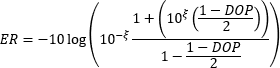
 ,
,takes into account the degree of polarization (DOP), which is the intensity of polarized light divided by the total light intensity.
References
[1] Chris Emslie, in Specialty Optical Fibers Handbook, edited by Alexis Mendez and T. F. Morse (Elsevier, Inc., New York, 2007) pp. 243-277.
[2] Edward Collett, Polarized Light in Fiber Optics (Elsevier, Inc., New York, 2007) pp. 45-53.
Date of Last Edit: Sept. 11, 2020
What is beat length and why is it often specified for PM fiber, instead of polarization extinction ratio?
It is difficult for manufacturers to specify a polarization extinction ratio (PER) for light output by polarization-maintaining (PM) fibers, since this parameter depends on the length of the fiber, how it is routed, and the polarization and alignment of the input light. Beat length is independent of these factors, which makes it a convenient parameter for quantifying the fiber's potential to preserve polarization. A smaller beat length is better, and it is a useful parameter to reference when choosing a PM fiber and its operating temperature. While beat length provides information about a PM fiber's potential to perform well, its actual performance and the PER of the light output by the fiber ultimately depend on the details of the fiber's deployment.
Click to Enlarge
Figure 1: The red and blue curves represent waves that are polarized parallel to the PM fiber's slow and fast axes, respectively. Since the slow axis has the higher refractive index, the wave polarized parallel to this axis (red wave) oscillates at a higher rate. This can be seen by looking at the waves' amplitudes (indicated by spheres) at differernt propagation distances.
Click to Enlarge
Figure 2: The amplitudes of the waves shown in Figure 1 are both plotted with respect to propagation distance (top). Note that distance illustrated in this figure is longer than the distance shown in Figure 1. Each wave's phase is plotted (middle) on a 0 to 2 scale, but in reality the two wave's absolute phases differ by a factor of 2. The difference between the waves' phase values (bottom, also shown on a 0 to 2 scale) increases linearly with distance.
The green diamonds on all three plots mark the points at which both waves share the same phase on a 0 to 2 scale. Between adjacent markers, the slow-axis wave accumulates an extra 2 in phase compared with the fast-axis wave. Note that this phase is generally not acquired over a whole number of periods. The beat length is the distance over which the accumulated phase difference is 2, and this is also the distance between adjacent markers.
Beat Length of a PM Fiber
The concept of a PM fiber's beat length can be visualized by considering waves propagating along the fiber's two orthogonal axes, fast and slow. One way these waves can be excited in the fiber is by coupling in monochromatic, linearly polarized light, with the input light's polarization angle oriented midway between the fiber's fast and slow axes.
If this is done, the orthogonally polarized waves will have the same amplitude and be in phase when they enter the fiber. But, the waves do not stay in phase as they propagate, since the refractive index of the slow axis is larger than that of the fast axis
The phase difference between the two waves increases linearly with propagation distance (Figure 2). Locations at which there is a factor of
The beat length (Lp ),

is proportional to wavelength () and inversely proportional to the fiber's birefringence
Typical Beat Lengths
The larger the refractive index difference between the two fiber axes, the larger the birefringence, the shorter the beat length, and the better the polarization-preserving performance of the fiber. The beat length remains constant along the length of the fiber, as long as the fiber's birefringence does not change. Manufacturers often specify beat length for selected wavelengths and limited temperature ranges.
To date, PM fibers with beat lengths <1 mm have had elliptical cores and mode field diameters (MFDs) significantly smaller than those of standard single mode optical fibers. Many applications require fibers with circular cores and MFDs close to those of standard single mode fibers. Typical PM fibers that meet these criteria and perform well have beat lengths between 1 mm and a few millimeters. It is interesting to note that standard single mode fibers also have measurable beat lengths, although they are meters long. This is due to their cores not having a perfectly circular cross section. Since the ellipticity of their cores is slight and changes randomly along the length of the fiber, standard single mode fibers are not useful as PM fibers.
The Amplitude Does not Beat
In the case of PM fibers, beat length refers to a repeating phase relationship between waves polarized parallel to the orthogonal slow and fast axes of a PM fiber. The sum of these waves at any point along the fiber determines the polarization state of the light beam at that point. For example, when the waves are in phase, the light is linearly polarized, and the waves are out of phase by /2 (90°), the light is circularly polarized.
An amplitude beat pattern does not occur, since these waves are polarized orthogonal to one another. Two waves only produce an amplitude beat pattern when they have components polarized parallel to one another. For the same reason, a signal with an interference term equal to zero will result when a photodetector is used to measure the combined intensity of two orthogonally polarized waves with different periods.
References
[1] Chris Emslie, in Specialty Optical Fibers Handbook, edited by Alexis Mendez and T. F. Morse (Elsevier, Inc., New York, 2007) pp. 243-277.
[2] Malcolm P. Varnham et al., "Analytic Solution for the Birefringence Produced by Thermal Stress in Polarization-Maintaining Optical Fibers," J. Lightwave Technol., LT-1(2), 332-339 (1983).
Date of Last Edit: July 30, 2021
Content improved by our readers!
Are polarization-maintaining fibers with stress rods affected by operating temperature?
Click to Enlarge
Figure 9: The PANDA PM fiber has stress rods embedded in its cladding. These cylinders are aligned parallel to the core. Since the glass of the stress rods contracts more than the surrounding cladding as the fiber cools from fabrication temperatures, the core is pulled in tension along the slow axis.
| Source of Change in Delay |
Change in Parameter | Resulting Change in Delay |
|
| Birefringence | Length | ||
Birefringence |
|
--- |
|
Fiber Length |
--- |  |
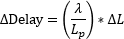 |

Click to Enlarge
Figure 11: Since the effect of the temperature-dependent birefringence dominates in Figure 10, the red trace from that figure is plotted alone to better show its range. These values were calculated using the assumption that the length of the fiber increases with temperature, while the fiber's birefringence remains constant with temperature.
Click to Enlarge
Figure 10: The relative delay (y-axis) between orthogonal polarization components propagating through a PANDA PM fiber changes as the fiber's temperature changes (x-axis). As the temperature increases, the polarization-maintaining performance decreases. Performance is improved by reducing the temperature. The blue and red traces were calculated using the assumption that only the birefringence or fiber length, respectively, changed with temperature.
The larger the refractive index difference between the orthogonal slow and fast polarization axes of a polarization-maintaining (PM) fiber, the better its PM performance. However, the magnitude of this difference (birefringence) decreases with increasing temperature, since the thermally dependent tension across the core drops with increasing temperature. The decrease in the fiber's birefringence is approximately proportional to the increase in temperature.
Temperature-Dependent Birefringence
Stress-birefringent PM fibers like PANDA and bow-tie fibers have stress rods embedded in their claddings (Figure 9). Since the stress rod's glass has a higher coefficient of thermal expansion (CTE) than the cladding's glass, the glass in the stress rods contracts at a higher rate than the rest of the cladding as the fiber cools immediately after fabrication. Due to their greater contraction, the stress rods pull on the surrounding cladding, which places the core under significant tension around room temperature. This creates birefringence in the fiber's core.
A proportionality constant ( ) relates the birefringence (B ),
 ,
,
to the difference between the temperature of the glass when it transitions between its liquid and glassy states (
Estimating the Impact of Temperature
If all of the light propagating in a PM fiber is polarized parallel to the same fiber axis, the polarization state of the light output by the fiber will be independent of temperature. If the light includes components polarized parallel to each of the fiber's axes, changing the operating temperature will change the elliptical polarization state of the light output by the fiber.
This is due to the relative delay between the two orthogonal components determining the output polarization state. That delay depends on the fiber's birefringence and the length of the fiber, which are both temperature dependent. But, only the change in birefringence significantly affects the fiber's polarization-maintaining performance.
Estimates of the relative significance of these two effects on the output polarization state were calculated using the equations in the table, a 1550 nm operating wavelength, and a 2 m length coefficient was assumed to be
The calculated results are plotted in Figures 10 and 11. The delay changes (y-axis), when the temperature changes (x-axis). This indicates that monitoring the temperature-dependent delay can provide information about the fiber's temperature-dependent birefringence and the fiber's potential to preserve polarization.
Temperature and Beat Length
While the fiber's birefringence determines the strength of a PM fiber's ability to preserve polarization, birefringence is not usually specified by the manufacturer. Beat length is a related and typically specified parameter. The beat length
is the ratio of wavelength () and birefringence and is shorter for higher-performance PM fibers. Note that for stress-birefringent PM fibers, beat length increases with temperature.
References
[1] Chris Emslie, in Specialty Optical Fibers Handbook, edited by Alexis Mendez and T. F. Morse (Elsevier, Inc., New York, 2007) pp. 243-277.
[2] Malcolm P. Varnham et al., "Analytic Solution for the Birefringence Produced by Thermal Stress in Polarization-Maintaining Optical Fibers," J. Lightwave Technol., LT-1(2), 332-339 (1983).
[3] Zhenyang Ding et al., "Accurate Method for Measuring the Thermal Coefficient of Group Birefringence of Polarization-Maintaining Fibers," Opt. Lett., 36(11), 2173-2175 (2011).
[4] M. Cavillon, P. D. Dragic, and J. Ballato, "Additivity of the coefficient of thermal expansion in silicate optical fibers," Opt. Lett, 42(18), 3650 - 3653 (2017).
Date of Last Edit: Sept. 16, 2020
Insights into Polarization
Scroll down or click on the following link to read about labels applied to polarized light, using a polarization ellipse to represent polarized light, and measuring the extinction ratio of polarizing optics.
- Labels Used to Identify Perpendicular and Parallel Components
- How is the polarization ellipse related to the polarization state?
- How is a Poincaré Sphere useful for representing polarization states?
- Can the extinction ratio of a polarizing component be measured using an unpolarized light source?
- Can a linearly polarized light source be used to measure the extinction ratio of a polarizing optic?
Labels Used to Identify Perpendicular and Parallel Components
| Labels | Notes |
|
|---|---|---|
| Perpendicular | Parallel | |
| s | p | Senkrecht (s) is 'perpendicular' in German. Parallel begins with 'p.' |
| TE | TM | TE: Transverse electric field. |
| ⊥ | // | ⊥ and // are symbols for perpendicular and parallel, respectively. |
| σ | π | The Greek letters corresponding to s and p are σ and π, respectively. |
| Sagittal | Tangential | A sagittal plane is a longitudinal plane that divides a body. |
Figure 1: Polarized light is often described as the vector sum of two components: one whose electric field oscillates in the plane of incidence (parallel), and one whose electric field oscillates perpendicular to the plane of incidence. Note that the oscillations of the electric field are also orthogonal to the beam's propagation direction.
When polarized light is incident on a surface, it is often described in terms of perpendicular and parallel components. These are orthogonal to each other and the direction in which the light is propagating (Figure 1).
Labels and symbols applied to the perpendicular and parallel components can make it difficult to determine which is which. The table identifies, for a variety of different sets, which label refers to the perpendicular component and which to the parallel.
The perpendicular and parallel directions are referenced to the plane of incidence, which is illustrated in Figure 1 for a beam reflecting from a surface. Together, the incident ray and the surface normal define the plane of incidence, and the incident and reflected rays are both contained in this plane. The perpendicular direction is normal to the plane of incidence, and the parallel direction is in the plane of incidence.
The electric fields of the perpendicular and parallel components oscillate in planes that are orthogonal to one another. The electric field of the perpendicular component oscillates in a plane perpendicular to the plane of incidence, while the electric field of the parallel component oscillated in the plane of incidence. The polarization of the light beam is the vector sum of the perpendicular and parallel components.
Normally Incident Light
Since a plane of incidence cannot be defined for normally incident light, this approach cannot be used to unambiguously define perpendicular and parallel components of light. There is limited need to make the distinction, since under conditions of normal incidence the reflectivity is the same for all components of light.
Date of Last Edit: Mar. 5, 2020
How is the polarization ellipse related to the polarization state?
Click to Enlarge
Figure 3: As the electric field ( ) propagates, the tip of the vector follows a helical path. In this case, propagation is along the z-axis, and the helicity of the path followed by the vector is positive (clockwise rotation).
Click to Enlarge
Figure 2: The electric field () can be expressed as the sum of two orthogonal components (Ex and Ey ), with a phase shift
Click to Enlarge
Figure 4: If an observer looks into the beam propagating from the origin in Figure 3, the tip of the rotating electric field vector traces out an ellipse. The ellipse can be described in terms of angles Ψ and χ. The equations in this figure use ( ) to represent (
  /λ - ωt ), where λ is the material-dependent wavelength, ω is frequency, and t is time.
The polarization ellipse is a way to visualize the polarization state.
As a laser beam propagates, the tip of its electric field vector moves along a three dimensional path determined by the polarization state. If an observer looking into the beam could see the electric field advancing in real time, the vector's tip would appear to cycle around the propagation axis while following a two-dimensional, elliptical track.
The shape of this track is the polarization ellipse, which becomes a line for linearly polarized light and a circle for circularly polarized light.
Components of Light
The electric field vector () can be described by its orthogonal components, Ex and Ey . Figure 2 illustrates a case of elliptically polarized light, in which the polarization is not linear or circular. The Ex and Ey components have different amplitudes, and the phase difference (δ ) between the Ex and Ey components is not an integer multiple of /2. The Ex and Ey components' values increase and decrease periodically, but they vary out of sync with one another and span different ranges.
If the orthogonal components were added together as vectors, the total field vector would rotate around the propagation axis as it traveled (Figure 3), and its length would vary with the rotation angle. Looking into the beam, perpendicular to the Ex - Ey plane, the tip of the vector would trace out the curve of the polarization ellipse (Figure 4).
Polarization Ellipse
An observer looking into the beam will describe a different polarization ellipse than an observer facing the opposite direction. Due to this, it is necessary to specify the direction the observer faces. Here, the observer is assumed to be looking into the beam.
The polarization ellipse is bound by a rectangle whose sides are equal to twice the amplitudes, Eox and Eoy , of the Ex and Ey components, respectively. This rectangle provides information about the fraction of the light contained in each orthogonal component.
To determine the specific characteristics of the polarization ellipse corresponding to a polarization state, the phase delay between the Ex and Ey components must also be considered. Key characteristics of the ellipse providing polarization state information are the rotation of the major axis with respect to the Ex axis and the relative lengths of the minor and major axes.
The angle (ψ ) between the major axis of the ellipse and the Ex axis is known by many names, including orientation angle, angle of inclination, rotation, tilt, and azimuth. It varies between -90° and 90°, and it is ±45° when Eox and Eoy have equal magnitudes.
The ellipticity of the polarization ellipse is the ratio (ε ) between the lengths of the minor and major axes. Since the orientation is typically stated as an angle, it can be convenient to also express ellipticity as an angle ( χ ). The ellipticity has a range of values from zero ( χ = 0°) for linearly polarized light, which is the case for δ = 0, to one ( χ = 45°) for circularly polarized light, which is the case for δ =  /2.
/2.
The tip of the electric field vector may rotate in a right-hand (clockwise) or left-hand (counterclockwise) direction as it propagates. This is known as the handedness or helicity of light, in which right-hand polarized light has positive helicity and left-hand polarized light has negative helicity. The direction can be determined using values of the E vector at time equal to zero (Et=0 ) and at a time one quarter of a period (T ) later (Et=T/4 ). If the cross product (

Click for Details
Figure 5: The ellipticity and orientation of the polarization ellipse provides information about the phase shift (δ ) between the Ex and Ey components of the electric field. The ellipses shown above result when the peak amplitudes of both components are the same. The direction of the E vector's rotation is indicated by the direction of the arrow on the polarization ellipse. Click the image to see ellipticity and orientation angles for each case.
Date of Last Edit: July 7, 2020
How is a Poincaré Sphere useful for representing polarization states?

Click to Enlarge
Figure 6: Polarization states are mapped to the Poincaré sphere using azimuthal and ellipticity angles, from the S1 axis and the equator, respectively. The state's radius is largest when the light is completely polarized (no fraction is unpolarized).
Click to Enlarge
Figure 7: States (blue circles) mapped to the equator (blue curve) of the spherical surface are perfectly linearly polarized. States (green circles) mapped to a value of ±1 on the S3 axis are circularly polarized. All elliptical polarization states that are not linearly or circularly polarized are mapped to other regions of the sphere.
Polarization states are mapped to the Poincaré sphere using an approach similar to the system of latitude and longitude used to locate points on the Earth's globe. The coordinates of points across and within the Poincarré sphere are specified using two angular values (azimuth and ellipticity) and a radius. The azimuth and ellipticity parameters are taken from the polarization ellipse representation of the polarization state. The radius is determined by the light's degree of polarization and has a maximum value of one, which corresponds to perfectly polarized light.
Both the Poincaré sphere and polarization ellipse are useful for visualizing a polarization state and observing its evolution. However, a key benefit of the spherical representation is that it simplifies the math needed to calculate incremental changes in polarization state.
Data Points on the Poincaré Sphere
The azimuthal angle /2/4
A radius of one corresponds to the surface of the sphere and indicates the light is completely polarized. The radius decreases as the fraction of unpolarized light increases. The degree of polarization (DOP) is the intensity of polarized light divided by the total light intensity.
The Stokes parameters (S1, S2, S3) of the polarization state correspond to the state's Cartesian coordinates (see the table below).
From One State to Another
Any two polarization state values plotted on the surface of the Poincaré sphere can be connected by a single arc, and the difference in the two states' azimuth and ellipticity can be calculated using spherical trigonometry. This provides a convenient way to predict the polarization state of light after interaction with a polarizing element, as well as to determine the azimuth and ellipticity of the polarizing element required to provide a desired polarization state.
| Cartesian to Poincaré Sphere Coordinates | |||
| S1 = cos(2χ)*cos(2ψ) | |||
| S2 = cos(2χ)sin(2ψ) | |||
| S3 = sin(2χ) | |||
| Selected Polarization States | Azimuth/2a | Ellipticity/2a | (S1, S2, S3) |
| Horizontal Linear | ψ = 0 | χ = 0 | (1, 0, 0) |
| +45° Linear | ψ =/4 |
χ = 0 | (0, 1, 0) |
| Vertical Linear | ψ = /2 |
χ = 0 | (-1, 0, 0) |
| -45° Linear | ψ = 3/4 |
χ = 0 | (0, -1, 0) |
| Right Circular | ψ = 0 | χ = /4 |
(0, 0, 1) |
| Left Circular | ψ = 0 | χ = -/4 |
(0, 0, -1) |
References
[1] Edward Collett, Polarized Light in Fiber Optics (Elsevier, Inc., New York, 2007) pp. 45-53.
[2] Russell A. Chipman, Wai-Sze Tiffany Lam, and Garam Young, Polarized Light and Optical Systems (CRC Press, New York, 2019) pp. 80-83.
Date of Last Edit: Sept. 11, 2020
Can the extinction ratio of a polarizing component be measured using an unpolarized light source?
The polarization extinction ratio of an optic under test (DUT) can be estimated by placing the DUT and a reference polarizer with a high extinction ratio between an unpolarized light source and an optical power sensor. This approach measures the maximum power to the minimum power that can be transmitted through the reference polarizer and DUT pair. The ratio of these two power measurements provides an accurate estimate of the DUT's extinction ratio when the extinction ratio of the reference polarizer is significantly higher than that of the DUT. If the reference polarizer and the DUT are linear polarizers of the same type (i.e. they have similar extinction ratios), this approach will provide an estimate that is ~50% of the DUT's actual extinction ratio. The estimate is expected to be ~99% of the DUT's extinction ratio when the reference polarizer's extinction ratio is two orders of magnitude higher than the DUT's.
Click to Enlarge
Figure 8: The extinction ratio of an optic under test (DUT) can be measured using the setup illustrated above. Unpolarized light is provided by a light emitting diode (LED), and both the DUT and a reference linear polarizer are placed between the source and power sensor. The lens tube, which is attached to the power sensor, helps block stray light from the power sensor. For illustrative purposes, it is assumed that the reference polarizer remains stationary, with its transmission axis oriented vertically. A value of Pmax is measured when the transmission axes of the DUT and reference polarizer are parallel (both vertical). A value of Pmin is measured when the transmission axes of the DUT and reference polarizer are perpendicular (i.e. when the DUT's transmission axis is horizontal). The dashed gold lines indicate the two orientations of the DUT's transmission axis that correspond to the two measurements.
Click to Enlarge
Figure 9: The difference between the measured value
Estimating the Extinction Ratio of the DUT
The experimental setup shown in Figure 8 can be used to estimate the DUT's extinction ratio (ERDUT ). Unpolarized light is transmitted through the reference linear polarizer, whose extinction ratio (ERref ) is known. The light is then transmitted through the DUT and measured by the detector.
An estimate of ERDUT can be calculated from two optical power measurements. One measurement is taken when the transmission axes of the reference polarizer and DUT are orthogonal (crossed). Crossing their axes minimizes the transmitted power
The other measurement records the optical power at the sensor when the two components' axes are parallel, which maximizes the amount of power
The ratio of Pmax and Pmin is ERest ,
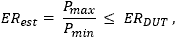
which provides an estimate of ERDUT . This estimate is more accurate when ERref is much larger than the ERDUT , as is discussed in a following section, Choose a High-ER Reference Polarizer. Note that ERest can never be larger than ERDUT , assuming the absence of noise and experimental error in the measurements.
It can be difficult to accurately measure Pmin , and measurement error can have a substantial negative impact on the value of ERest . Following some guidelines can provide the first steps to improving the accuracy of low-power-signal measurements.
It is important to note that this approach estimates the absolute extinction ratio of the DUT, rather than the extinction ratio of the light.
Reference Linear Polarizer's Placement
If the source light can be considered unpolarized, Pmax and Pmin can be measured with the DUT preceding or following the reference polarizer in the beam. In addition, it will not matter whether the DUT, the reference polarizer, or both are rotated to orient their axes parallel or perpendicular to one another. This can be seen by referencing an equation,
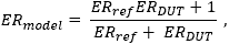
which was derived by multiplying the Mueller matrices for two partial polarizers. The derivation assumed both polarizing components are imperfect, so that they transmit some light polarized perpendicular to their transmission axes. This is realistic, since only ideal polarizers with infinite extinction ratios transmit no light polarized perpendicular to their transmission axes. The value (ERmodel ) computed by the equation models the measured value (ERest ), when the light source is completely unpolarized. The values of ERref and ERDUT cannot be less than 1, and a value of 1 describes a neutral density filter. [1]
It should be noted that many sources described as being unpolarized actually emit some polarized light. If this is the case, the degree of polarization (DOP) is not zero, and the measurement constraints and equations are different than those described here. One way to investigate the source's DOP is to remove the DUT from the setup in Figure 8 and monitor the detected optical power while rotating the linear polarizer around the optical axis. If the detected power does not vary as the linear polarizer rotates, the source can be considered unpolarized. If the power variation is detectable above the power meter's noise floor, the source should be considered partially polarized.
Choose a High-ER Reference Polarizer
It is important to choose a reference polarizer with an extinction ratio that is significantly higher than that of the DUT. As illustrated by the equation for ERmodel , whose calculated values are plotted as the blue curve in Figure 9, the value of ERest is theoretically restricted from exceeding the lower of the two components' extinction ratios. In addition, the value of ERmodel only approaches the actual value of the DUT's extinction ratio when ERref is orders of magnitude higher than ERDUT . Note that when the reference and DUT polarizers have nearly equal extinction ratios, which is notably typical when the reference polarizer and DUT are the same type of polarizer, ERmodel is ~50% of ERDUT .
The red squares plotted in Figure 9 are experimental data (ERest ). The measurements were made using linear polarizers with known extinction ratios, in which one polarizer was assigned to be the reference linear polarizer and the other was the DUT.
If a reference polarizer with a suitably high extinction ratio is not available, that polarizer can be combined with others into a set. Assemble these polarizers that their transmission axes are all exactly parallel to one another. Then, the effective extinction ratio of this set (ERset ) is the product of the polarizers' individual extinction ratios, and ERset should be used in place of ERref in calculations.
References
[1] Michael Kraemer and Tom Baur, "Extinction ratio measurements on high purity linear polarizers," Proc. SPIE Polarization: Measurement, Analysis, and Remote Sensing XIII, 10655, 1065505 (2018).
Date of Last Edit: May 16, 2021
Can a linearly polarized light source be used to measure the extinction ratio of a polarizing optic?
The extinction ratio of an optical component under test (DUT) can be measured using light from a laser or other linearly polarized source, but it is often necessary to insert a linear polarizer between the source and the DUT. The linear polarizer is needed when the light from the source has an extinction ratio that is not significantly higher than the extinction ratio of the DUT, which is frequently the case. Obtaining an accurate measurement of the DUT's extinction ratio requires the incident light's extinction ratio to be substantially higher than the DUT's. Inserting one or more linear polarizers between the source and the DUT is one way to improve the extinction ratio of the light incident on the DUT.
Click to Enlarge
Figure 10: The extinction ratio of the optic under test (DUT) can be estimated from two optical power measurements. One, Pmax , requires the transmission axis of the DUT to be parallel with the polarization direction of the incident light, which is vertical in this illustration. The second measurement, Pmin , requires the DUT's transmission axis to be perpendicular (crossed with) the incident light's polarization direction. The estimate's accuracy is better when the extinction ratio of the light incident on DUT is much higher than the DUT's extinction ratio. One or more linear polarizers inserted between the source and DUT may be needed to improve the light's extinction ratio, since light from lasers described as linearly polarized often has an extinction ratio too low to achieve the desired accuracy.
Click to Enlarge
Figure 11: The difference between the measured value
Estimating the Extinction Ratio of the DUT
It is important to note that this approach estimates the absolute extinction ratio of the DUT, rather than the extinction ratio of the light.
Accurately estimating a DUT's extinction ratio requires linearly polarized incident light, whose extinction ratio is much higher than that of the DUT, as well as an optical power sensor. It is sometimes the case that a linearly polarized source provides light whose extinction ratio is adequate (see the discussion in the following section), but it is typically necessary to include one or more linear polarizers between the source and DUT (Figure 10).
Two optical power measurements are needed to estimate the DUT's extinction ratio. The measurement of the maximum power (Pmax ) transmitted to the power sensor requires the DUT's transmission axis to be oriented parallel to the polarization direction of the incident light. The measurement of the minimum power (Pmin ) transmitted by the DUT requires the DUT's transmission axis to be oriented perpendicular to the polarization direction of the incident light. These two orientations of the DUT's transmission axis are indicated by the dashed gold lines in Figure 10, assuming the polarization direction of the source light is vertical.
The ratio of Pmax and Pmin is ERest ,
whose value can be used to estimate the DUT's extinction ratio
It can be difficult to accurately measure the values of Pmin , and errors in these measurements can have a substantial negative impact on the value of ERest . Following some guidelines can provide the first steps to improving the accuracy of low-power-signal measurements. Note that an unpolarized source can also be used to measure the extinction ratio of a DUT.
Improve the Extinction Ratio of the Source Light
The extinction ratio of the light incident on the DUT can potentially limit the value of ERest to a value substantially less than ERDUT . The value of ERest only approaches the value of ERDUT when the extinction ratio of the incident light is significantly higher than the extinction ratio of the light incident on the DUT. For example, when the extinction ratio of the incident light equals the value of ERDUT , ERest is only ~50% of the value of ERDUT . When the extinction ratio of the incident light is two orders of magnitude higher than ERDUT , ERest is ~99% of the value of ERDUT .
In general, the extinction ratio of light from most lasers is too low to be suitable for measuring the extinction ratios of highly polarizing DUTs, such as linear polarizers. In this case, a linear polarizer placed before the DUT (as shown in Figure 10) can improve the extinction ratio of the incident light. By the same principle, adding an additional linear polarizer at this location will further improve the extinction ratio. The transmission axes of the two polarizers should be aligned exactly parallel to obtain the highest extinction ratio.
Effect of Improving the Incident Light's Extinction Ratio
The value of ERest can be modeled for sources with different extinction ratios as well as configurations that do and do not include linear polarizer(s) between the source and the DUT. The modelled value (ERmodel ),
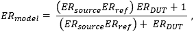
is plotted as the blue curve in Figure 11. This equation assumes a single linear polarizer is placed between the source and DUT, and that the extinction ratio of the source is ERsource . The value of ERsource is set to 1 when the source is unpolarized. The extinction ratio of this polarizer is ERref . If a set of polarizers is used instead, the value ERref should be replaced with the set's effective extinction ratio. If there are no polarizers located between the source and the DUT, replace ERref with a value of 1.
If the positions of the linear polarizer and the DUT are switched, so that the DUT is placed closest to the source, the effect can be modeled by exchanging the ERDUT and ERref variables in this equation. This change worsens the model's (and the measurement's) estimate of ERDUT . For best results, the set of linear polarizers should be located closest to the source.
References
[1] Michael Kraemer and Tom Baur, "Extinction ratio measurements on high purity linear polarizers," Proc. SPIE Polarization: Measurement, Analysis, and Remote Sensing XIII, 10655, 1065505 (2018).
Date of Last Edit: May 16, 2021
Insights into Optical Reflectors
Scroll down or click on one of the following links to read about recommended mirror diameters, as well beam paths through a retroreflector and gold-coated retroreflector prisms.
- Is there a rule for choosing the mirror's diameter based on the laser beam's diameter?
- How does alignment affect the beam path through a retroreflector?
- Why coat the backsides of solid prism retroreflectors with metal?
- Does the angle of incidence affect the output beam power from a corner-cube retroreflector?
Is there a rule for choosing the mirror's diameter based on the laser beam's diameter?
The diameter of the laser beam should be significantly smaller than the clear aperture of the mirror (Figure 1). A general rule restricts the diameter of the beam to no more than a third of the mirror's diameter. This limits the risk of introducing aberrations into the beam, which will occur if it interacts with the coating boundary near the perimeter of the surface and / or is clipped by the edge of the optic.

Click to Enlarge
Figure 1: The clear aperture of the mirror should have a larger diameter than the beam. A general rule recommends the mirror's diameter be at least a factor of three larger than the beam's 1/e2 diameter.
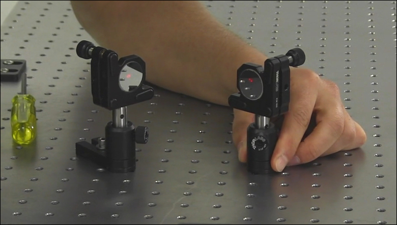
Click to Enlarge
Figure 2: A larger-diameter mirror provides the flexibility to preserve optical beam quality despite situations in which the laser spot is not perfectly centered on the mirror or is elongated due to oblique incidence.
Beam Diameter and Optical Power
When the laser beam has a Gaussian intensity profile, it is common to measure its diameter across the 1/e2 intensity points. If a visible wavelength beam is observed, the 1/e2 diameter generally appears to enclose the beam. However, the intensity of the beam is 13.5% of the peak intensity along the 1/e2 perimeter, and there is measurable power beyond this diameter.
A mirror would optimally have a diameter (D ) large enough to reflect all of the beam's power. The fraction of the reflected optical power (PT ),
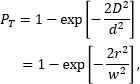
can be calculated using D and the 1/e2 beam intensity diameter (d ), or using the mirror's radius (r ) and the 1/e2 beam intensity radius (w ). [1]
When the diameter of the mirror is a factor of 1.52 larger than the beam's 1/e2 diameter, the mirror can reflect 99% of the power. Increasing the mirror's diameter to twice the beam's diameter will reflect over 99.96% of the power. If the beam is not perfectly centered on the mirror, the fraction of reflected light will be lower.
Beam Position and Clear Aperture
The mirror's optical performance is specified over the area of the clear aperture, which typically includes all but a thin annulus around the perimeter of the mirror. It is good practice to confine the laser beam to the clear aperture, since nothing is known about the mirror's performance in the surrounding region. In addition, a beam that extends beyond the clear aperture risks being clipped by the edge of the mirror.
If the mirror's diameter is twice the beam's diameter, and the beam is perfectly centered on the mirror, the optical quality of the beam will be preserved and approximately all of the beam power will be reflected. However, any misalignment will impact beam quality. A larger mirror diameter provides additional flexibility during alignment and accommodates situations in which the beam is not perfectly centered in the clear aperture. Due to this, it can be more convenient to work with mirrors that have clear apertures at least a factor of three larger than the beam diameter.
Want additional Insights on beam alignment?
Watch the full video.
Reference
[1] Bahaa E. A. Saleh and Malvin Carl Teich, Fundamentals of Photonics (John Wiley & Sons, Inc., New York, 1991) p. 85.
Date of Last Edit: Oct. 12, 2020
How does alignment affect the beam path through a retroreflector?
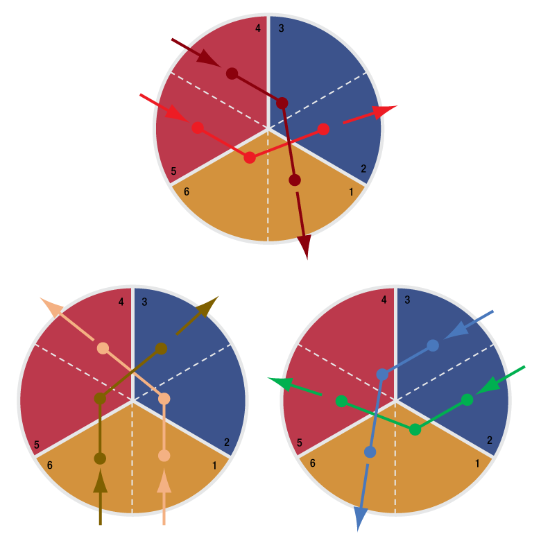
Click to Enlarge
Figure 4: There are six possible sequences of reflections for a beam. The zone in which the first reflection occurs determines the sequence. These maps apply to beams approximately parallel with the retroreflector's normal axis. The beam paths are indcated by arrows, and dots mark reflections.
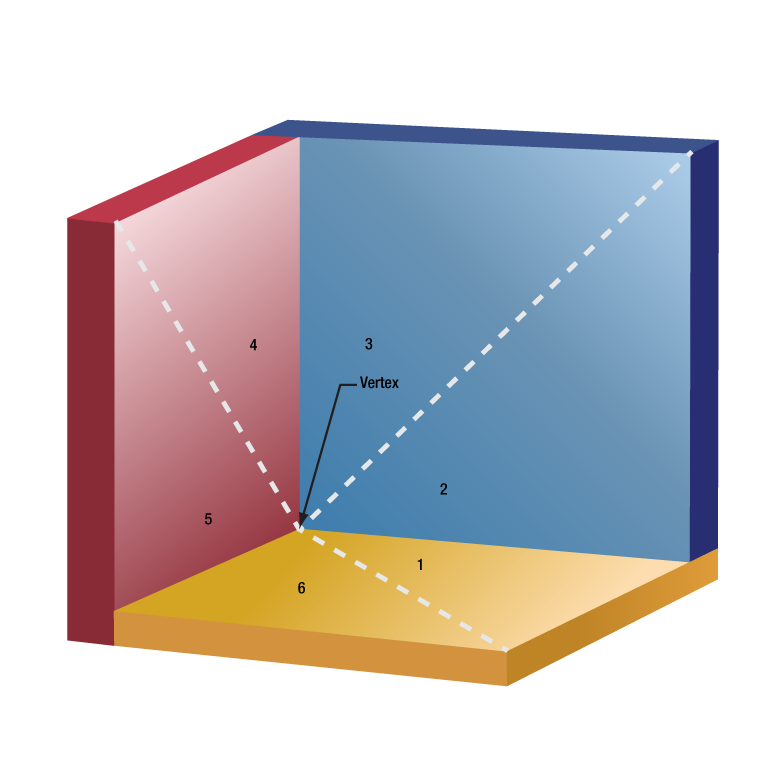
Click to Enlarge
Figure 3: The three reflective faces of a corner-cube retroreflector are shown in false color and with numerical labels assigned to each half. Retroreflectors are designed to reflect an incident beam once from each face and provide an output beam parallel to the input.

Click to Enlarge
Figure 6: Shifting the position of the first reflection to below the diagonal of the red face causes the next reflection to occur from the yellow face. After the third reflection, from the blue face, the beam exits the retroreflector travelling parallel to but shifted from the output beam in Figure 5.
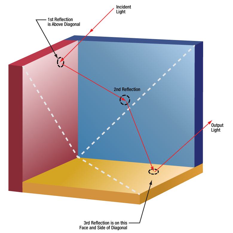
Click to Enlarge
Figure 5: When the first reflection occurs above the diagonal of the red face, and the beam is parallel to the retroreflector's normal axis, the second reflection occurs from the blue face. The beam then reflects from the yellow face before exiting the retroreflector.
Beams output from corner-cube retroreflectors travel parallel to the input beam, but in the opposite direction. The input beam can be aligned to the vertex or to a point on one of the three faces. The input and output beams are colinear if the input beam is aligned to the vertex. The two beams will be separated if the input beam spot does not overlap the vertex.
Input beams aligned to one of the retroreflector's faces will reflect from that face and then the other two before exiting the retroreflector. For a range of incident angles, there are six possibilities for the order in which the beam will reflect from the three different faces. lt can be useful to select the path through the retroreflector for reasons that include optimal beam positioning and minimizing polarization effects.
For a beam to follow a particular sequence of reflections, it is not sufficient to align the beam so that it is incident on a specific face. The beam must also be incident on the proper half of that face.
Tracing the Beam Path
When looking into the vertex of the retroreflector, reflective effects make it possible to see the six halves of the three faces. Here, they are identified using dashed diagonal lines (Figure 3). In addition, the three faces of the retroreflector are shaded with false color for illustrative purposes. The normal axis is not shown, but it passes through the vertex and is equidistant from all three faces.
The six different possible reflection sequences can vary with angle of incidence. The maps in Figure 4 apply to beams nearly parallel with the normal axis. While a hollow retroreflector is used for these illustrations, these sequences of reflections also apply to prism retroreflecting mirrors.
The position of the first reflection determines which sequence of reflections the beam will follow through the retroreflector. The beam always exits from a different face than it entered.
Example
Figures 5 and 6 illustrate the two orders of reflections that can occur when the first reflection occurs from the left-most vertical face. The incident beam is parallel to the retroreflector's normal axis.
When the first reflection occurs above the diagonal, as shown in Figure 5, the last reflection occurs from the horizontal (yellow) mirror. However, locating the first reflection below the diagonal results in a last reflection from the other vertical (blue) mirror. The output beams of these two cases are parallel to, but shifted from, one another.
Date of Last Edit: July 8, 2020
Why coat the backsides of solid prism retroreflectors with metal?
Click for Details
Figure 8: Vertically polarized beams were input to a TIR solid prism retroreflector (PS975M) and a backside-gold-coated solid prism retroreflector (PS975M-M01B). The polarization ellipse of each output beam is shown in the zone that provided the beam's third reflection. For a plot of the ellipticity angle ( χ ) and orientation angles ( ψ ) with respect to the horizontal axis, click here.
Click to Enlarge
Figure 7: Horizontally polarized beams were input to a TIR solid prism retroreflector (PS975M) and a backside-gold-coated solid prism retroreflector (PS975M-M01B). The polarization ellipse of each output beam is shown in the zone that provided the beam's third reflection. For a plot of the ellipticity angles ( ψ ) with respect to the horizontal axis, click here.
Click to Enlarge
Figure 10: Retroreflectors convert some of the input light to the orthogonal polarization. Over 90% of the light output from the backside-gold-coated solid prism retroreflector (PS975M-M01B) remained polarized in the input state. In the case of the TIR solid prism retroreflector (PS975M), that percentage strongly depended on beam path and did not exceed 80%.
Click to Enlarge
Figure 9: A retroreflector is designed to reflect an input beam once off of each face. When the beam is approximately normal to the viewing plane illustrated in Figures 7 and 8, the beam will follow one of six beam paths.
When the backsides of solid prism retroreflectors are coated with metal, polarization changes induced in the output beam are significantly reduced.
This is due to the difference between specular reflections, which occur from interfaces between glass and the higher refractive index metal, and reflections that occur due to total internal reflection (TIR), which require the backside material, like air, to have a lower refractive index.
Compared with TIR, a specular reflection from a glass-metal interface better preserves the input beam's polarization ellipticity.
Polarization and Beam Path Diagrams
Beam paths through a retroreflector can be described by dividing its three reflective faces into six wedge-shaped zones (Figures 7, 8 and 9). Solid gray boundary lines mark physical lines of contact between reflective faces. Dotted gray lines indicate boundaries between the halves of each face.
The retroreflectors in these figures are oriented with one face-to-face interface aligned with the vertical axis. When the input beam is normal to these figures' viewing planes, Figure 9 describes the order in which the input beam reflects from the three faces before being output.
Output Polarization State
Two sets of six measurements were made for both a PS975M TIR solid prism retroreflector and a
In Figures 7 and 8, the polarization states of the output beam are represented using polarization ellipses. Each output beam's polarization ellipse is shown in the zone that provided the third reflection.
Ideally, the output beam would have the same polarization state as the input beam. However, these measurements indicate the retroreflectors converted some of the incident light to the orthogonal polarization. The plot in Figure 10 is a measure of the fraction of light in the output beam that was polarized parallel to the input.
The backside-gold-coated solid prism retroreflector was significantly more successful in maintaining the polarization state of these linearly polarized input beams.
Date of Last Edit: July 7, 2020
Does the angle of incidence affect the output beam power from a corner-cube retroreflector?
Click to Enlarge
Figure 12: Since the refractive indices of glass and air are different, the beam reflects at the front face. Reflected light can make multiple passes through the retroreflector before being output. Coherent overlapping beams produce interference effects.
Click to Enlarge
Figure 11: The beam path through a corner-cube retroreflector includes a reflection from each of the three back faces, in an order determined by the position of the incident beam. The incident beam shown above has a 0° AOI and is displaced from the vertex.
The beam power output by solid prism retroreflectors may oscillate around an average value as the angle of incidence (AOI) varies. This is due to a multiple-beam interference effect that can occur when the coherence length of the light source is at least twice the optical path length through the retroreflector.
When the front face of a solid retroreflector has an anti-reflective coating, oscillation amplitudes for all AOIs are substantially reduced. Hollow metal-coated retroreflectors provide output beams whose power is approximately independent of AOI.
Beam Path
These corner-cube retroreflectors provide an output beam that travels in a direction parallel and opposite to the incident beam. Figure 11 shows one beam path.
The AOI is determined using a reference axis normal to the front face of the retroreflector. This axis passes through the vertex and is equidistant from the three back faces.
Reflections from the Front Face
As illustrated in Figure 12, light can make multiple passes through a solid prism retroreflector, depending on whether the light reflects from or is transmitted through interfaces between the front face and the surrounding medium.
When a glass retroreflector is surrounded by air, ~96% of the light is in the primary output beam, which makes a single pass through the retroreflector, and ~0.16% is in the beam that completes an additional round trip. In this work, light making additional round trips had negligible intensity.
Conditions for Interference
Since the output of solid prism retroreflectors consists of beams that have travelled different optical path lengths, they will interfere if:
- The beams overlap, which is more likely when the AOI of the incident beam is near 0° and the output is measured closer to the retroreflector. At larger distances, the beam deviation specified for the retroreflector and the AOI will more widely separate the first- and third-pass beams.
- The coherence length of the source is longer than the difference in path length between the primary beam and the overlapping beam that has made more than one pass through the retroreflector.
Click to Enlarge
Figure 14: Output power as a function of AOI differed depending on the type of corner-cube retroreflector. Data from measurements, made as described in Figure 13, were normalized to the same scale, and traces were vertically shifted as a visual aid. Oscillation amplitude was strongly suppressed when the front face was AR-coated
Click to Enlarge
Figure 13: The power output by a TIR solid prism retroreflector (PS975M) was measured as a function of AOI. The incident beam was provided by a DBR1064S 1064 nm laser source, whose coherence length was several meters. The largest-amplitude oscillations resulted around 0° AOI, where the first- and third-pass beams overlapped. The 1/e2 beam diameters did not overlap for AOIs larger than ±1° at a distance of 30 cm from the front face of the retroreflector.
Corner-Cube Retroreflectors Compared
The variation of output power with small AOI was compared for four different types of corner-cube retroreflectors: a PS975M TIR solid prism retroreflector, a
Figure 131 plots the normalized measurements made for the TIR solid prism retroreflector. As the AOI increased, the centers of the first- and third-pass beams shifted away from one another. At AOIs greater than around ±1°, the beams' 1/e2 diameters no longer overlapped. This resulted in the oscillation amplitude decreasing with AOI. The range of AOIs over which oscillations were significant would increase if the detector were located closer to the front face.
Figure 14 plots the trace from Figure 13, as well as traces measured for the other three retroreflectors, on the same scale but vertically shifted as a visual aid. These results indicate that an antireflective-coated front face suppresses power oscillations in beams output by solid prism retroreflectors. The power output by hollow retroreflectors does not oscillate, since there is no material boundary at the front face.
Date of Last Edit: July 7, 2020
DM713 Digital Micrometer: LabVIEW and C# Programming References
Click to Enlarge
Figure 1: Visual C# and LabVIEW programs can be written to interrogate the DM713 Digital Micrometer. Examples are detailed in programming references available for download.
Programming references that provide introductions to communicating with the DM713 Digital Micrometer (Figure 1) are available. One reference has been developed for LabVIEW, and the other for Visual C#. Each reference includes a step-by-step discussion for writing the program, as well as a section that concisely provide the full program text without explanation.
Included in the LabVIEW Programming Reference:
- Instructions for downloading and installing the driver software.
- Information concerning the required cabling and connecting to the DM713's COM port.
- Creation of a new VI that establishes serial communications with the DM713.
- Data from the DM713 is continuously received.
- The displacement value and its units of measurement are displayed.
- Logging a data value in response to a button click is implemented.
Included in the Visual C# Programming Reference:
- Information for connecting the computer to the DM713's COM port.
- Instructions for spawning a secondary thread to continuously communicate with the DM713.
- Procedure for operating on the received data, to extract the displacement value and units.
- Instructions for displaying the displacement values and units in the program's GUI.
- Logging a displacement value to a file in response to a button click.
Date of Last Edit: Dec. 4, 2019
Photonics How-To Videos Providing Insights Into Getting Things Done in the Lab
Sometimes the best way to learn is by watching someone else. Thorlabs offers these videos to share tips, tricks, and methods we find ourselves frequently using in the lab. If you have any questions, please contact Tech Support.
Laser Alignment and Setup:
- How to Align a Laser
- Align Fiber Collimators to Create Free Space Between Single Mode Fibers
- Setting Up a TO Can Laser Diode (Viewer Inspired)
- Setting up a Pigtailed Butterfly Laser Diode (Viewer Inspired)
Polarization:
- Align a Linear Polarizer's Axis to be Vertical or Horizontal to the Table
- Align a Linear Polarizer 45° to the Plane of Incidence
- Create Circularly Polarized Light Using a Quarter-Wave Plate (QWP)
- Distinguish the Fast and Slow Axes of a Quarter-Wave Plate
- Build a Polarimeter to Find Stokes Values, Polarization State (Viewer Inspired)
- New! How Light’s Incident Angle Affects Transmission & Finding Brewster’s Angle
Optics and Optical Devices:
- Build a Solar Imaging Telescope with Tracking Capability
- Collimate a Laser with a Shear-Plate Collimation Tester (Viewer Inspired)
- Use Laser Speckle to Find the Beam Focus
- Optical Power Meter Parameter Setup for Improved Accuracy
- Align an Off-Axis Parabolic (OAP) Mirror to Collimate a Beam (Viewer Inspired)
- Calibrate a Spatial Light Modulator (SLM) for Phase Delay (Viewer Inspired)
- Herriott Cell Setup and Configuration (Viewer Inspired)
- Collimate Light from an LED
- How to Align an Optical Isolator
Fiber Optics:
- Cleave a Large-Diameter Silica Fiber Using a Hand-Held Scribe
- PM Fiber Measurements Used to Align Incident Polarization State (Viewer Inspired)
- Measure the Insertion Loss of a Fiber Optic Component
- Align FiberPorts on a FiberBench (Viewer Inspired)
Optomech:
- Tips for Bolting Post Holders to Optical Tables, Bases, and Breadboards
- Mounting your Optomech: Bases, Post Holders, and Posts
- How to Motorize a Manual Translation Stage
- Working with KF (QR) Vacuum Flange Components
- Working with CF Vacuum Flanges
Software Tutorials:
- Visual Studio® Project Setup and C# Programming - Kinesis® BBD300 Series
- Raster Scan Using Visual Studio® and C# Programming - Kinesis® BBD300 Series Controller
- Camera Setup and Image Acquisition Using Visual Studio® and C# Programming
- Python® Automation of a Rotation Mount and Power Meter (Viewer Inspired)
Date of Last Release: May 7, 2024
How to Align a Laser
Two methods for aligning a laser beam so that it propagates parallel to the surface of the optical table are demonstrated.
The first technique adjusts the pointing angle of a laser, whose tip and tilt can be adjusted. Using a ruler, the laser beam is leveled and directed along a row of tapped holes in the table.
Starting with this aligned beam, the technique for changing both the direction and the height of a beam from a fixed laser source is demonstrated. Two mirrors, which are set at different heights, direct the beam along another row of tapped holes in the table. The beam is then leveled at the height of the second mirror using two irises.
| Products Featured During Demonstration | ||
| Laser Module | Kinematic Mounts | Irises |
| Adapter (Laser to Mount) | Mirrors | Ruler |
Date of Last Edit: Sept. 8, 2020
|
Right Click to Copy Link to this Section |
1 |
Optical Power Meter Parameter Setup for Improved Accuracy
An optical power meter should be configured specifically for the light incident on the power sensor. Three important optical power meter parameters to set are the center wavelength of the light, the maximum optical power the sensor will measure, and the zero offset resulting from the detection of ambient light.
The procedure for setting these three parameters, and some things to consider while configuring them, are demonstrated and discussed.
Always follow your institution's laser safety guidelines. Unlike the low-power source used in this demonstration, other laser sources may be damaged by back reflections. Many stray reflections, which can endanger colleagues and the laser, can be avoided by blocking the laser beam when it is not needed.
| Products Featured During Demonstration | ||
| Optical Power Meter | Optical Power Sensor | Fiber-Coupled Laser Source |
Date of Last Edit: Sept. 24, 2020
|
Right Click to Copy Link to this Section |
2 |
How to Motorize a Manual Translation Stage
The procedures for replacing the manual adjusters on a couple of translation stages with motorized actuators are demonstrated. Using the techniques described here allows the adjuster to be exchanged without damaging the stage.
The first example uses a MT1B linear translation stage with a 0.5" travel range. The adjuster screw is swapped for a ZFS13B stepper-motor-driven actuator. In the second half of the video, the micrometer on an XR25P linear translation stage with a 1" travel range is replaced by a DC-servo-motor-driven actuator.
In addition, the video provides an introduction to best practices for mounting these stages to a table or breadboard and demonstrates the use of the locking plate.
| Products Featured During First Half of Demonstration | Products Featured During Second Half of Demonstration | |||
| Linear Translation Stage | Stepper-Motor-Driven Actuator | Linear Translation Stage | DC-Servo-Motor-Driven Actuator | |
Date of Last Edit: Nov. 11, 2023
|
Right Click to Copy Link to this Section |
3 |
Tips for Bolting Post Holders to Optical Tables, Bases, and Breadboards
A common, unfortunate result of securing a post holder to a base or optical table is threads poking up through the bottom of the post holder. These exposed threads limit the height adjustment range offered by the post holder. Additional frustrations can result after rotating the post in the post holder, since this can unintentionally screw the post onto the exposed threads.
The solution is to keep screw length in mind when selecting a setscrew or cap screw to secure a post holder. In this video, observe consequences unfold due to threads projecting up from the bottom of the post holder, and learn techniques for overcoming this problem. The options of securing a post holder to a base or directly to the table are also compared.
A sequel to this Video Insight provides tips for using optomechanical components to build a stable foundation under an optical setup, as well as to avoid accidental damage to the components.
| Products Featured During Demonstration | |||||
| Ø1/2" Post Holders | Ø1/2" Posts | Mounting Base | Iris | Cap Screws | Setscrews |
Date of Last Edit: Apr. 28, 2022
|
Right Click to Copy Link to this Section |
4 |
How to Align an Optical Isolator
Align a Faraday isolator to ensure optimal transmission of optical power from the source, as well as effective suppression of reflections traveling back towards the source. Alignment is demonstrated using a polarization-dependent free-space isolator with a 510 nm to 550 nm operating range and a linearly polarized and collimated 520 nm laser.
These optical isolators output linearly polarized light and provide best performance when the input beam is linearly polarized.
Always follow your institution's laser safety guidelines. Unlike the low-power source used in this demonstration, other laser sources may be damaged by back reflections. Many stray reflections, which can endanger colleagues and the laser, can be avoided by blocking the laser beam when it is not needed.
| Products Featured During Demonstration | ||
| Free-Space Isolator | Power Sensor | Post Collar |
| Laser | Power Meter | Balldrivers and Hex Keys |
Date of Last Edit: Sept. 10, 2020
|
Right Click to Copy Link to this Section |
5 |
Align a Linear Polarizer's Axis to be Vertical or Horizontal to the Table
The beam paths through many optical setups are routed parallel to the optical table. When this is the case, both the plane of incidence and the p-polarization state are typically oriented parallel to the table's surface, while the s-polarization state is perpendicular. Therefore, polarizers aligned to pass p- or s- polarized light effectively have their axes aligned to be parallel or perpendicular, respectively, to the table's surface.
A procedure for optically aligning the axis of a polarizer to be perpendicular to the optical table is discussed and demonstrated using optical power readings of light transmitted through the polarizer. Then, three options for aligning the axis of a polarizer to be parallel to the table are outlined. The method of crossed polarizers is demonstrated. Tips and tricks for obtaining more precise measurements are also shared.
| Products Featured During Demonstration | |||
| Collimated Laser | Polarizing Beam Splitter | Optical Power Sensor | Post Collar |
| Linear Polarizers | Precision Rotation Mounts | Power Meter | Ruler |
Date of Last Edit: Oct. 23, 2020
|
Right Click to Copy Link to this Section |
6 |
Cleave a Large-Diameter Silica Fiber Using a Hand-Held Scribe
An optical-quality end face can be achieved when a large-diameter optical fiber is manually cleaved using a hand-held scribe. The procedure is demonstrated using a multimode fiber with a 400 µm diameter core.
After stripping the protective polymer buffer from the end of the fiber and securing the fiber to a flat surface, a hand-held scribe is used to score the top surface of the fiber. The scribe should create a shallow nick in the fiber's cladding, away from the fiber's core. When cleaving smaller-diameter fibers, avoid creating too deep of a nick by reducing the scribing force and sweeping motion. In some cases, it is sufficient to lightly press a stationary scribe to the fiber. Applying a longitudinal tension to the fiber, across the nicked region, cleaves the fiber.
Also demonstrated is the visual evaluation of the end face quality using an eye loupe. A good quality end face will be a flat plane, perpendicular to the fiber's long axis. The light output from the cleaved end face was also observed on a viewing screen, and tips are shared for inspecting the output light distribution for information about the quality of the end face.
| Products Featured During Demonstration | ||||
| Fiber Buffer Stripping Tool | Fiber Grippers | Quick-Release Adjustable Fiber Clamp | SMA Bare Fiber Terminator | 10X Eye Loupe |
| Ruby Scribe | Fiber-Coupled LED | Free-Standing Platform | Pillar Posts | Viewing Screen |
Date of Last Edit: Nov. 3, 2020
|
Right Click to Copy Link to this Section |
7 |
Measure the Insertion Loss of a Fiber Optic Component
Insertion loss measures the drop in optical power caused by the addition of a device to a fiber optic network. All sources of optical loss contribute to a device's insertion loss, including reflections, absorption and scattering due to intrinsic material properties, micro- and macrobending losses, split ratios, splice loss, and connector loss.
A single-ended insertion loss measurement is demonstrated. In this approach, a reference cable is attached to the source, and then the power at the cable's output is measured. Next, a mating sleeve is used to attach the component under test to the reference cable. The optical power at the selected output port of the component is measured. The insertion loss is calculated by first taking the ratio of this power reading to the power measured at the reference cable output, and then expressing the ratio in terms of decibels (dB).
The single-ended insertion loss measurement includes the loss from coupling light into the device, which is often mostly due to the misalignment of the fiber cores in the mating sleeve. However, this measurement does not include the same type of loss that occurs when coupling the light output from the device into the next leg of the fiber optic network. Note also that the insertion loss is wavelength dependent and will differ for each combination of device input and output ports selected for the measurement. This is due to the differences in split ratio, bend loss, absorption, scattering, reflections, and all other individual sources of attenuation along the optical path between the two ports.
| Products Featured During Demonstration | |||||
| Fiber-Coupled Laser Source | Mating Sleeve | Power Sensor | Power Meter | 50:50 Coupler | Single Mode Patch Cables |
Date of Last Edit: Dec. 3, 2020
|
Right Click to Copy Link to this Section |
8 |
Create Circularly Polarized Light Using a Quarter-Wave Plate (QWP)
Circularly polarized light can be generated by placing a quarter-wave plate in a linearly polarized beam, provided a couple of conditions are met. The first is that the light's wavelength falls within the wave plate's operating range. The second is that the wave plate's slow and fast axes, which are orthogonal, are oriented at 45° to the direction of the linear polarization state. When this is true, the incident light has equal-magnitude components parallel to the wave plate's two axes. The wave plate delays the component parallel to the slow axis by a quarter of the light's wavelength (/2) with respect to the component parallel to the fast axis. By creating this delay, the wave plate converts the polarization state from linear to circular.
An animation at the beginning of the demonstration illustrates the results of aligning the input linear polarization state with the wave plate's fast axis, slow axis, and angles in between. The perspective used to describe the angles and orientations is looking into the source, opposite the direction of light propagation. The procedure is then demonstrated for orienting input and output polarizers to define the reference orthogonal polarization directions, as well as provide polarization-dependent power measurements. The wave plate is placed between the two polarizers, and the effects of different orientations are explored. The quality of the circularly polarized light output by the wave plate is checked by rotating the second polarizer's transmission axis. The light's polarization is closer to circular when the power reading fluctuates less during rotation.
| Products Featured During Demonstration | ||||
| HeNe Laser | Quarter-Wave Plate | Precision Rotation Mounts | Power Sensor | Power Meter |
| Optical Isolator (for HeNe) | Linear Film Polarizers | V-Clamp Mount | SM1 Thread Adapter (for Power Sensor) | SM1 Lens Tube |
Date of Last Edit: Dec. 30, 2020
|
Right Click to Copy Link to this Section |
9 |
Align a Linear Polarizer 45° to the Plane of Incidence
The transmission axis of a linear polarizer can be set at a 45° angle to the plane of incidence, with the help of two additional linear polarizers. The two supporting polarizers are aligned so that one's axis is parallel and the other's is perpendicular to the plane of incidence. Orienting the transmission axis of the third polarizer at a 45° angle to the plane of incidence is done by rotating the transmission axis to make 45° angle with the axes of the polarizer pair.
This is demonstrated for the case in which the plane of incidence is parallel to the optical table. The procedure used to align the first polarizer's axis parallel to the table requires repeatedly rotating the polarizer 180° around the vertical axis. The linear polarizer assemblies have rectangular bases, and the fixed position retainer (fork) provides a fixed corner reference on the table. The fork allows the polarizer assembly to be quickly and precisely placed after flipping it around the vertical axis. Following each 180° flip, the transmission axis of the polarizer is first rotated by hand and then finely tuned using the mount's integrated micrometer (mic). After the first polarizer's axis is aligned, the second polarizer's axis is then crossed with it. When this is done, the light transmitted by the second polarizer is minimized.
The third polarizer is then placed between the other two polarizers and its transmission axis is rotated. The rotation angle affects the optical power transmitted by this set of three polarizers, and the throughput is maximized when the angle is 45° with the plane of incidence. One way to check the result, as well as determine the maximum possible power that can be obtained at the detector, is to use the cosine squared (Malus') law. It calculates the power output by a linear polarizer when the incident light is linearly polarized.
| Products Featured During Demonstration | |||
| Laser Module | Precision Rotation Mounts | Power Sensor | Power Meter |
| Linear Film Polarizers | Fixed Position Retainer (Fork) | SM1 Thread Adapter (for Power Sensor) |
SM1 Lens Tube |
Date of Last Edit: Jan. 19, 2024
|
Right Click to Copy Link to this Section |
10 |
Align Fiber Collimators to Create Free Space Between Single Mode Fibers
Two collimators, inserted into a fiber optic setup, provide free-space access to the beam. The first collimator accepts the highly diverging light from the first fiber and outputs a free-space beam, which propagates with an approximately constant diameter to the second collimator. The second collimator accepts the free-space beam and couples that light into the second fiber. Some collimation packages, including the pair used in this demonstration, are designed for use with optical fibers and mate directly to fiber connectors.
Ideally, 100% of the light emitted by the first fiber would be coupled into the second fiber, but some light will always be lost due to reflections, scattering, absorption, and misalignment. Misalignment, typically the largest source of loss, can be minimized using the alignment and stabilization techniques described in this video.
In this demonstration, the first fiber is single mode. The optical power incident on the second collimator, as well as the power output by the second fiber, are measured. When the second fiber is multimode with a 50 µm diameter core, alignment resulted in 91% of the power incident on the second collimator being measured at the fiber output. This value was 86% when the second fiber is single mode. Some differences in collimator designs, and their effects on the characteristics of the collimated beams, are also discussed.
| Products Featured During Demonstration | ||||
| Fiber-Coupled Laser | Kinematic Mounts | Fiber Adapter Cap (for Power Sensor) |
Single Mode Patch Cable (FC/PC) | Fiber Cable Storage Reels |
| Triplet Fiber Optic Collimators | Power Sensor | Power Meter | Hybrid Single Mode Patch Cable | 2" Posts |
| Adapter (Mount-to-Collimator) |
SM1 Thread Adapter (for Power Sensor) |
Fiber Connector Cleaner | Step-Index Multimode Patch Cable | 0.5" Post Holders |
Date of Last Edit: April 1, 2021
|
Right Click to Copy Link to this Section |
11 |
Setting Up a TO Can Laser Diode (Viewer Inspired)
Installing a TO can laser diode in a mount and setting it up to run under temperature and current control presents many opportunities to make a mistake that could damage or destroy the laser. This step-by-step guide includes tips for keeping humans and laser diodes safe from harm.
Protection from the considerable risk of electrostatic discharge (ESD) is provided by an ESD strap, but only if the strap is grounded and worn correctly. Wearing the strap as demonstrated makes it easier to keep the strap's metal plate in constant skin contact. Moisturizing the skin with lotion formulated for use in electronic and cleanroom environments can also help.
A laser diode can be damaged by attempting to force it into a socket that is the wrong size. To avoid this, find a suitable mount by referencing the physical dimensions of the pins identified in the video. Since current flow in the wrong direction is also dangerous to laser diodes, it is critical to correctly orient the laser in the socket, as well as properly set the polarity of the mount's switches. Current drivers typically also have a polarity setting. The diode orientation and mount and driver settings can be determined using information included in the laser's pin diagram and electrical diagram, whose symbols are decoded and explained in the video.
Excessive operating temperatures and drive current are both risks that can be mitigated using correctly configured current and temperature controllers. Their setup is demonstrated. The proper use of two frequently misunderstood parameters, maximum power and maximum current, in configuring the current driver is also shown.
| Products Featured During Demonstration | ||||
| TO Can Laser Diode | ESD Strap | Current Controller | Integrating Sphere Power Sensor | Flexure Clamping Base |
| Laser Diode Mount | Laser Safety Glasses | Temperature Controller | Power Meter | Tweezers |
Date of Last Edit: May 7, 2021
|
Right Click to Copy Link to this Section |
12 |
Setting Up a Pigtailed Butterfly Laser Diode (Viewer Inspired)
A laser diode packaged in a butterfly housing can be precisely controlled, in a compact package, when the laser is installed in a mount that includes thermoelectric cooler (TEC) and current drivers. The mount can make it easier, and safer, to operate the laser, but the procedure for installing the laser in the mount and configuring the settings requires some care. This video provides a step-by-step guide, which begins with an introduction to the different components and concludes with the laser operating under TEC control and with the recommended maximum current limit enabled.
This demonstration is also filled with useful details that can be forgotten in bulleted lists describing the setup procedure. These include tips for wearing an ESD strap, determining when to use thermal grease, applying the right amount of thermal grease, creating good electrical connections between the laser's pins and mount, easing the removal of the laser from the mount, safeguarding the fiber pigtail of the installed laser, cleaning an angled physical contact (APC) fiber connector, using the Steinhart-Hart thermistor values provided on the laser spec sheet, and making power measurements to determine the laser's current limit setting.
Date of Last Edit: June 17, 2021
|
Right Click to Copy Link to this Section |
13 |
Distinguish the Fast and Slow Axes of a Quarter-Wave Plate
A wave plate has two axes, and light polarized parallel to the slow axis is delayed more than light polarized parallel to the orthogonal fast axis. The wave plate's retardance determines the delay difference. A couple of crossed polarizers can be used to locate an axis (Video Insight) but cannot identify the axis as fast or slow. However, by including a mirror in the setup and comparing optical power measurements with calculated values, it is possible to distinguish between the fast and slow axes of a quarter-wave plate. Note that this technique cannot be used to distinguish the fast and slow axes of a half-wave plate.
The video includes an overview of the measurement setup and discussion of the conventions used to align and orient the optical components. The accurate interpretation of the results depends on these details, including whether the transmission axes of the generating and analyzing polarizers are parallel or orthogonal (crossed). Crossed polarizers are used in this demonstration, in contrast to a paper [1] that also describes the technique.
The fast and slow axes of the quarter-wave plate are identified by comparing measurements of the power transmitted through the system to a pair of theoretical curves. The Fresnel reflection equations, as well as other equations, needed to compute these curves are provided. The refractive index of the reflective surface is required to generate these curves. Be aware that complex refractive indices can be written with a positive or a negative sign before the imaginary part, depending on the preferred convention. While either option is compatible with this approach, the chosen sign affects the interpretation of the curves. In this demonstration, the positive-sign convention was chosen.
| Products Featured During Demonstration | ||||
| HeNe Laser | Quarter-Wave Plate | Unprotected Gold Mirror | Power Sensor | Power Meter |
| Optical Isolator (for HeNe) | Linear Polarizers | Kinematic Mirror Mount | SM1 Thread Adapter (for Power Sensor) |
SM1 Lens Tube |
| V-Clamp Mount | Precision Rotation Mounts | Iris | Balldrivers | Quick-Release Lens Tube Adapter |
[1] Petre C tlin Logoftu, "Simple method for determining the fast axis of a wave plate," Opt. Eng. 44, 3316-3318 (2002).
Date of Last Edit: July 30, 2021
|
Right Click to Copy Link to this Section |
14 |
Visual Studio® Project Setup and C# Programming - Kinesis® BBD300 Series Controller
Starting a program and initializing connected devices can be one of the largest hurdles to writing code that remotely controls a device. This tutorial for Thorlabs' Kinesis® software package provides step-by-step instructions for using C# and the .NET framework to create a new Visual Studio® project and initialize connected devices, which in this case is a BBD300 series motor controller connected to a two-axis stage. A basic move sequence is then added to the program and used to test the execution of the code.
The demonstration begins with instructions for creating a new Visual Studio project and adding the required dynamic link libraries (DLLs). In this example, there is one connected controller. The program is written to execute its two-step initialization process, since the controller's chassis and channels must be initialized individually. Each channel connects to one axis of a connected stage.
In this demonstration, one of the controller's two channels is initialized, allowing the two-axis stage to be moved in one direction. Custom velocity and position settings are specified for the move command, and instructions are included to perform the disconnect shutdown sequence after the move sequence is completed. Try-catch blocks are added to the code to provide instructions to the program in the case that an error is thrown by a method. Command and position status information is made available to the user, and status messages are printed to the PC's console screen.
These steps are used as the foundation of a program described in another Video Insight that executes a stepped, bidirectional raster scan using the same controller and XY stage. The code demonstrated during this video can be downloaded from Thorlabs' official GitHub account.
| Products Featured During Demonstration | |||
| Kinesis Software Package | Two-Axis Brushless DC Controller | XY Scanning Stage | Slide / Petri Dish Holder for Inverted Microscopes |
Date of Last Edit: Nov. 17, 2021
|
Right Click to Copy Link to this Section |
15 |
Build a Polarimeter to Find Stokes Values, Polarization State (Viewer Inspired)
A polarimeter, which is an optical tool used to measure the polarization state of light, can be constructed using linear polarizers, a quarter-wave plate, and an optical power sensor and meter. This video describes two methods for building a manual polarimeter, the classical method and the rotating wave plate method, and then uses both to measure a laser beam's polarization state. [1] Both approaches provide measurement data that describe the polarization state in terms of the four Stokes parameters. This demonstration includes discussion of the relationships between the Stokes parameters and different polarization states, including linearly and circularly polarized light.
In this demonstration, polarization handedness is defined with respect to time and from a perspective of looking into the beam, back towards the source. This video illustrates this convention by visualizing a fixed viewing plane oriented perpendicular to the propagating beam. As the beam passes through the plane, the beam's instantaneous polarization vector traces out a shape on the plane. The shape is traced out as a function of time, and the direction in which the shape is traced corresponds to the handedness of the light. The shape itself is the polarization ellipse, which is a convenient and common way to describe light's polarization state. The relationship between the polarization ellipse and the Stokes parameters is also discussed.
Prior to filming, the transmission axes of the linear polarizers and wave plate used to build these polarimeters were oriented with respect to the table. The following descriptions link to Video Insights demonstrating the alignment procedures:
- Align a linear polarizer horizonal or vertical with respect to the table.
- Align a linear polarizer at 45° with respect to the table.
- Align a wave plate's axis to be horizontal with respect to the table.
- Determine whether a wave plate's axis is fast or slow.
| Products Featured During Demonstration | ||||
| HeNe Laser | Quarter-Wave Plate | Power Sensor | Power Meter | Fixed Position Retainer (Fork) |
| Optical Isolator (for HeNe) | Linear Polarizers | SM1 Thread Adapter (for Power Sensor) |
SM1 Lens Tube | Optical Post Assemblies |
| V-Clamp Mount | Precision Rotation Mounts | Iris | Quick-Release Lens Tube Adapter | Balldrivers |
[1] Beth Schaefer, Edward Collett, Robert Smyth, Daniel Barrett, and Beth Fraher "Measuring the Stokes polarization parameters," Am. J. Phys. 75, 163-168 (2007).
Date of Last Edit: Oct. 19, 2021
|
Right Click to Copy Link to this Section |
16 |
Raster Scan Using Visual Studio® and C# Programming - Kinesis® BBD300 Series Controller
A benefit of motorized XY stages is that they can be remotely controlled to execute a patterned scan, such as a raster scan, across a specified area. This tutorial for Thorlabs' Kinesis® software package provides step-by-step instructions for writing a program for a BBD300-series motor controller that moves the connected two-axis stage in a stepped, bidirectional raster scan pattern. The program is written using C#, the .NET framework, and the Visual Studio® development environment.
This tutorial builds on the foundation established by the previously released Video Insight, Visual Studio Project Setup and C# Programming - Kinesis BBD300 Series Controller. After providing a brief overview of different raster scan patterns and approaches, this demonstration quickly reviews some of the steps included in the Visual Studio Project Setup tutorial. This includes referencing libraries, configuring the project platform, and initializing the controller's chassis and two channels.
Three types of move methods are implemented. One is used to home a chosen stage axis, and another is used to move the stage to a specific position. The third implements a jog, which moves the stage along a particular axis by a specified step size. The raster scan is implemented by first moving the stage to an initial position, and then executing a series of jogs along the stage's X- and Y-axes. An example of debugging the code is shown, and the stepped, bidirectional raster scan is successfully executed.
The code demonstrated during this video can be downloaded from Thorlabs' official GitHub account.
| Products Featured During Demonstration | |||
| Kinesis Software Package | Two-Axis Brushless DC Controller | XY Scanning Stage | Slide / Petri Dish Holder for Inverted Microscopes |
Date of Last Edit: Nov. 17, 2021
|
Right Click to Copy Link to this Section |
17 |
Align an Off-Axis Parabolic (OAP) Mirror to Collimate a Beam (Viewer Inspired)
Off-Axis parabolic (OAP) mirrors are often used to collimate divergent beams, but aligning these mirrors can be a frustrating experience. This is because there are multiple variables that must be controlled during the alignment process. This demonstration divides the procedure into discrete steps and includes helpful tips for successfully positioning the mirror and light source. In addition, the dependence of the correct alignment on the mirror's geometry is discussed, and the typical effects of different misalignment geometries on the beam shape are shown on a viewing screen.
In this demonstration, the divergent output of an optical fiber and an OAP mirror are aligned so that the incident light and the collimated reflected beam travel in a plane parallel to the surface of the optical table. Because of this, an important initial step in the procedure is to set both the height of the source and the center of the mirror mount's bore at the height of the desired collimated beam. Then, an iterative approach is used in which the mirror is rotated to bring the plane of reflection parallel to the plane of the table, and the fiber's end face is moved to the mirror's focal point.
| Key Components | Additional Products Featured During Demonstration | ||||
| Aluminum OAP Mirror | Post Collars | SMA-SMA Patch Cable | Viewing Screen (Smaller) | Spanner Wrench | |
| SM1-Threaded Adapter (for OAP Mirror) |
Fiber-Coupled LED | Lens Mount | Viewing Screen (Larger) | Magnetic Button Clamps | |
| SM1-Threaded Mirror Mount | T-cube LED Driver | SM1-Threaded Fiber Adapter | Ruler | 1/4"-20 Cap Screw Kit | |
Date of Last Edit: Dec. 14, 2021
|
Right Click to Copy Link to this Section |
18 |
Camera Setup and Image Acquisition Using Visual Studio® and C# Programming
When a scientific camera is integrated into a setup, it can be convenient to automate image acquisition and storage using a hardware trigger. This can be enabled using the software development kit (SDK) provided with Thorlabs' scientific cameras. The use of the SDK to control the operation of a scientific camera is demonstrated using a custom Visual Studio® console application written in C#, as well as a setup that includes a scientific camera, light emitting diode (LED), LED driver, and PC.
The demonstration begins with a general overview of the setup, and then steps through the settings needed to configure the LED driver to pulse the LED five times while providing a TTL output signal each time. Pulsing the light source is one approach to limiting a sample's total light exposure, and the TTL signal can be used to synchronize image acquisition with the illumination of the sample. A cable couples the TTL hardware trigger to the camera.
A blank Visual Studio console application is then opened, and the code is explained as it is typed line-by-line. The program finds all available cameras connected to the PC and is used to select one, whose parameters the program will configure for the setup. The exposure time is set to be slightly less than the LED pulse duration, and a single image acquisition is specified to occur when a hardware trigger is received. Each image is saved to a file as a bitmap, and the total number of acquired images is limited to five. The demonstration concludes with the successful execution of the program, which results in five saved image files that were each taken during a separate flash of the LED.
The code demonstrated during this video can be downloaded from Thorlabs' official GitHub account.
File Paths to DLLs and Supporting Documentation:
- Location of DLLs added during project setup: C:\Program Files\Thorlabs\Scientific Imaging\Scientific Camera Support\Scientific Camera Interfaces
- Detailed documention including camera's supported features: C:\Program Files\Thorlabs\Scientific Imaging\Documentation\Scientific Camera Documents
Date of Last Edit: Jan. 25, 2022
|
Right Click to Copy Link to this Section |
19 |
Align FiberPorts on a FiberBench (Viewer Inspired)
This video demonstrates a complete procedure for aligning two FiberPorts on a FiberBench. The procedure takes into account the coupled functionality of the various adjustment screws, such as the Zθ screws. Adjusting any of the three Zθ screws individually affects both the angular orientation and Z-axis position of the lens. When all three Zθ screws are adjusted as a set, it is possible to move the lens such that the final position corresponds to only a change in angular orientation or shift in position along the Z-axis.
For example, adjusting each of the three Zθ screws by the exact same amount in the same direction translates the lens along the Z-axis without affecting the lens's angular orientation. The different techniques used to complete this and other adjustments are shown during the demonstration, so that this alignment procedure can be customized according to preference.
Before aligning the FiberPorts to one another, the lens in each should be pre-aligned to collimate light from a coupled optical fiber. The pre-alignment step should not be necessary if the FiberPort has not been used, since FiberPorts are provided pre-aligned. The alignment procedure begins by tuning the X-axis and Y-axis adjusters and progresses to the Zθ adjusters. To avoid complicating the alignment procedure, it is recommended that the X- and Y-axis adjuster positions are not changed after beginning work with the Zθ adjusters.
The optical power collected by the coupling fiber is used to monitor the progress of the alignment procedure. However, it should be noted that a drop in power after an adjustment may not indicate a misstep in the procedure. Instead, the drop may correspond to a local minimum en route to a global maximum. This demonstration provides tips for interpreting and investigating the progress of the alignment, as well as advice for making consistent adjustments.
| Key Components | Additional Products Featured | ||||
| FiberPorts | SM1 Thread Adapter (for the Power Sensor) |
(FC/PC to FC/PC) |
Fiber Connector Cleaner | ||
| Power Sensor | Adapter Cap |
Single Mode Patch Cable (FC/PC to FC/APC) |
|||
| Irises (Pillar Post and Flexure Clamping Base Used in Free-Standing Iris Assembly) |
Power Meter | Multimode Patch Cable |
Ruler | ||
Date of Last Edit: Feb. 15, 2022
|
Right Click to Copy Link to this Section |
20 |
Working with KF (QR) Vacuum Flange Components
A vacuum connection between two KF flanged components is made by compressing an O-ring between the two flanges. Minimizing leak rates through this vacuum coupling requires the flat flange faces to be smooth and clean, as well as the O-rings to be malleable and undamaged. This video demonstrates methods for coupling and disconnecting KF flanged components and shares tips for handling, maintaining, and assembling these popular vacuum flanges. Vacuum systems that include KF flanges can generally support vacuum levels down to 10-8 Torr (
There are many benefits to using KF flanged components in vacuum systems, including a genderless design, standardized sizes, quick decoupling and reconnection times, and being relatively inexpensive. Many of these features are made possible by the elastomeric O-ring that serves as a gasket.
The effectiveness of the vacuum seal depends on several factors including the conditions of both flange faces and the O-ring, the compression applied to the O-ring, and the O-ring's history of temperature exposure and usage. Excessive amounts of compression (>60%) and exposure to high temperatures increases the rate at which the O-ring develops compression set. Compression set is a term used to refer to permanent changes in the O-ring's shape, which includes stiffening of the elastomeric material. Inspecting the O-ring and flange surfaces as shown in the video, and then replacing damaged components and stiffened O-rings can optimize performance. The application of vacuum grease to an O-ring is also demonstrated, and guidance for determining whether or not to use vacuum grease is provided.
| Products Featured During Demonstration | ||
| Wing Nut Clamp (KF25) | Blank Cap (KF25) | Nitrile Gloves |
| O-Ring and Carrier (KF25) | Elbow and Straight Pipes (KF25) | Solvent Dispenser and Wipes |
Date of Last Edit: June 10, 2022
|
Right Click to Copy Link to this Section |
21 |
Mounting your Optomech: Bases, Post Holders, and Posts
Optical setups are typically built upon a foundation of optomechanical components like posts, post holders, and bases. There are different approaches to designing and building the foundation. Some result in optical setups that are more affected by vibrations and more likely to be misaligned when bumped. In addition, certain techniques used to assemble components can accidentally damage them.
Unfortunately, it is typically necessary to build the entire setup to observe the effects of different approaches, so evaluating the benefits and disadvantages of each can be difficult or time consuming. In addition, the existence of other approaches may not be obvious, since it can be easy to avoid thinking about components that are as familiar as posts, post holders, and bases. The techniques presented in this video are methods we have found useful and should provide a good starting point for working with optomech.
This demonstration shines a spotlight on these common building-block components and includes tips learned though long experience designing and working with them. The purpose and use of features that may have escaped notice, such as the relief cut on bases, the through hole in optical posts, and the benefits of washers are revealed. Guidelines for choosing post and post holder heights to increase mechanical stability are provided, as well as suggestions for avoiding damage to kinematic mounts when attaching a post. This video also demonstrates a potentially unexpected approach for mounting larger components, which uses two post holders, two posts, and a base.
Additional tips for avoiding unintended consequences and preserving the full adjustment height when bolting post holders to optical tables, bases, and breadboards are demonstrated in this Video Insight.
| Products Featured During Demonstration | ||
| Posts | Compact Mirror Mount | 8-32 Hardware Kit Also Available: M4 Hardware Kit |
| Post Holder | Mirror Mount | 1/4"-20 Hardware Kit Also Available: M6 Hardware Kit |
| Mounting Base | Laser Diode Mount | Balldriver Caddy Kit, Imperial Also Available: Balldriver Caddy Kit, Metric |
Date of Last Edit: Apr. 29, 2022
|
Right Click to Copy Link to this Section |
22 |
Use Laser Speckle to Find the Beam Focus
When a lens is mounted in a lens tube, optic mount, or cage plate, the exact position of the lens within the fixture may not be known, which can make it difficult to accurately predict the location of the beam focus and align the system. One approach to finding the beam focus with respect to the fixture uses laser speckle.
During this demonstration, laser speckle is used to find focal points provided by lenses mounted in individual lens tubes. After locating the focus of each mounted lens, the distance between the focal point and the external shoulder of each lens tube is measured.
The mounted lenses are then used to construct a Keplerian beam expander, using a design in which empty lens tubes are inserted between the two mounted lenses. The required total length of the lens tubes separating the two mounted lenses is estimated using the previously measured distances to the focal points. This approach avoids tedious trial-and-error that can result when the beam expander is constructed by first guessing the required total lens tube length, and then iteratively measuring beam quality and adjusting the length until achieving the desired result.
A transmissive glass diffuser is used during this demonstration to create the speckle pattern. The size of the speckle is largest when the ground surface of the diffuser is at the focus, where the beam size is smallest. It is recommended that the beam is incident on the ground face of the diffuser. This allows direct measurement of the distance to the focus, without needing to take the diffuser's optical thickness into account. After assembling the beam expander, a shearing interferometer is used to fine-tune the collimation of the expanded beam.
| Products Featured During Demonstration | |||
| Optical Diffuser | Compact Laser Module | Ø1" Lens Tubes | Dovetail Optical Rail |
| DIY Adapter (Diffuser to Slip-Ring Mount): Lens Tube Coupler and Retaining Ring |
Adapter (Laser to Mount) | Adjustable Ø1" Lens Tubes | Optical Rail Carrier |
| Threaded Kinematic Mount | Slip-Ring Mount | Post Collar | |
| Plano-Convex Lenses | Fiber Storage Reel | Digital Calipers | Ruler |
| Shearing Interferometer | Viewing Screen | Retaining Ring Wrench | V-Groove Block |
Date of Last Edit: June 6, 2022
|
Right Click to Copy Link to this Section |
23 |
Python® Automation of a Power Meter and Rotation Mount (Viewer Inspired)
A Python script that automates control of a Kinesis® K-Cube™ motor controller and a power meter is written using Visual Studio® Code. The program acquires optical power measurements from the power meter as the rotation mount's angle sweeps through 180°, which is required to characterize a variable optical attenuator. Since this code uses libraries developed using the .NET framework, running this code requires Python.NET to be installed.
This tutorial implements the code specific to the K-Cube motor controller first, followed by the code for the power meter. The packages and classes required by both devices are identified, and the steps required to initialize and complete shutdown for both devices are shown. In addition, an approach is described for acquiring power readings and checking controller status while the motor is moving. The Python script is executed once after the K-Cube section of the code is complete, and a second time after the program is finished.
The K-Cube motor controller and power meter were automated in order to characterize the optical power transmitted through a pair of fixed, crossed linear polarizers when a rotating half-wave plate is located between them. As the half-wave plate rotates, the polarization orientation of the light transmitted by the output polarizer remains constant, while the transmitted power varies sinusoidally. Measurements of this transmitted optical power, as well as the corresponding rotation angles of the mount in which the half-wave plate is secured, are provided by the program.
The code written using Visual Studio Code during this video can be downloaded from Thorlabs' official GitHub account.
| Products Featured During Demonstration | ||||
| Motion Control Software | Compact Laser Module | Manual Rotation Mount | Power Sensor | Slip-Ring Mount |
| K-Cube Motor Controller | Adapter (Laser to Mount) | Linear Polarizers | Power Meter | Mounting Base |
| Motorized Rotation Stage | Threaded Kinematic Mount | Wave Plates | Ø1" Lens Tubes | Storage Reel |
Date of Last Edit: Jul. 26, 2022
|
Right Click to Copy Link to this Section |
24 |
Working with CF Vacuum Flanges
A vacuum coupling that supports operation at ultra-high-vacuum levels
Damage to the knife edge, an aggressive approach to tightening the bolts, and reusing gaskets can all result in leaky CF vacuum couplings. The techniques demonstrated in this video reduce the risk presented by these factors, which are all related to the limited malleability of the metal gasket. It is important that the knife edges are in pristine condition, since the gasket is not soft enough to fill narrow or abrupt features, such as a nick in a knife edge. An approach of gradually and iteratively tightening the bolts is effective in maintaining a uniform thickness of the gasket around its circumference, while tightening each bolt all at once can result in thickness variations in the gasket that are difficult or impossible to flatten. This is a consequence of the metal gasket’s limited ability to flow and can result in gaps between the gasket and knife edges. Using a new gasket is always recommended. Even a gasket that was only partially compressed during a previous use may not be malleable enough, when reused, to conform to the contours of the knife edges. This is because compression has the effect of strain (work) hardening the metal.
While a leaky vacuum connection can result in time lost to leak checking and re-opening the vacuum system to locate and fix the problem, productive work can also be delayed as a result of broken or malfunctioning components in or attached to the chamber. Due to this, an overview of special considerations for handling and using fiber feedthroughs is also included in this video.
ConFlat® is a registered trademark of Agilent Technologies, Inc.
| Products Featured During Demonstration | |||
| Optical Fiber Feedthrough | 1/4-Hard Copper Gaskets | Fiber Inspection Scope | Nitrile Gloves |
| UHV Fiber Patch Cable | Solvent Dispenser | Fiber Connector Cleaner | Wipes |
Date of Last Edit: Sept. 21, 2022
|
Right Click to Copy Link to this Section |
25 |
Calibrate a Spatial Light Modulator (SLM) for Phase Delay (Viewer Inspired)
The phase delay (phase modulation) provided by a reflective liquid crystal on silicon spatial light modulator (SLM) depends on a number of things, including the applied control voltage, ambient conditions, and the characteristics of the incident light. When a manufacturer calibrates the SLM’s phase delay as a function of the applied voltage, the calibration is typically performed under specific operating conditions and for collimated light with a particular wavelength and angle of incidence. Since an application’s setup and operating conditions can differ significantly from the manufacturer's, it is often beneficial to recalibrate the SLM’s phase delay for each application.
This Video Insight demonstrates an interferometric method [1] for calibrating the phase delay of reflective SLMs that are designed to modulate the phase without affecting the linear polarization state of the incident light. The calibration setup requires only a collimated, linearly polarized input beam and a camera, in addition to the SLM.
When working with SLMs, it is common to represent phase delay patterns using grayscale values, in which each shade of gray represents a specific phase delay. Calibration determines the specific phase delay provided for each grayscale value, under the current operating conditions. This calibration approach applies a uniform phase delay to one half of the SLM's panel. This half is referred to as the mirror side and provides a reflected beam. A binary phase grating is applied to the other half, which provides a diffracted beam. The reflected and -1st order diffracted beams overlap and create interference fringes, which are monitored during the calibration procedure. The voltage applied to the mirror side of the SLM is varied across the full range, and the fringes shift each time the applied voltage changes. The fringe shift is directly related to the change in phase delay.
A second video made to accompany this Video Insight provides additional background information about the optical properties of the liquid crystal layer. The effects of the applied voltage on the liquid crystal layer’s refractive index are illustrated, as well as the effects of the layer on linearly polarized light with different polarization orientations. Note that the SLM provides unexpected results when the linearly polarized light is not aligned parallel with what is often called the SLM's optic axis, which is actually the rotation plane of the molecules in the liquid crystal layer.
[1] José Luis Martínez Fuentes, et al., "Interferometric method for phase calibration in liquid crystal spatial light modulators using a self-generated diffraction-grating," Opt. Express. 24, 14159 - 14171 (2016).
Date of Last Edit: Nov. 29, 2023
|
Right Click to Copy Link to this Section |
26 |
Collimate a Laser with a Shear-Plate Collimation Tester (Viewer Inspired)
A shear-plate collimation tester is a compact shearing interferometer that is convenient for inserting into a beam path. When in place, the device can be used to test and optimize a laser beam’s collimation. This Video Insight demonstrates a technique for using the device, shares some troubleshooting tips, and provides guidance for determining whether the approach is a good option for testing the collimation of a particular beam.
The device can remain in the beam while the position of the collimating lens, which in this case is an achromatic doublet, is adjusted. Fringes visible on the ground glass diffuser, which is on top of the device, indicate whether the beam is converging, diverging, or collimated.
It should be kept in mind that this technique requires light with sufficient coherence, low wavefront aberrations, and a shear plate thickness compatible with the beam diameter. Note also that the distance over which a beam is collimated is never infinite, so the device should be located within approximately one Rayleigh range of the collimated beam's waist.
Assistance is provided for diagnosing the problem when no interference fringes are visible, or the fringes are difficult to interpret. The demonstration shows when the solution is to use a thinner shear plate, to adjust the lens position, or to add a magnified viewer to the top of the device. It is also shown that a different method is required to test and optimize beam collimation when there are significant wavefront aberrations or an insufficient coherence length.
Date of Last Edit: Mar. 22, 2023
|
Right Click to Copy Link to this Section |
27 |
PM Fiber Measurements Used to Align Incident Polarization State
Polarization-maintaining (PM) fiber can only preserve the polarization state of input light that is both linearly polarized and correctly aligned to one of the two PM fiber's axes. Due to this, setups for coupling light into a PM fiber often include a linear polarizer and some means for rotating the orientation of the input polarization state. This Video Insight demonstrates two methods for aligning linearly polarized input light. The first approach uses a polarimeter, and the second uses a linear polarizer in front of a power sensor. Both approaches require smoothly increasing or decreasing the fiber’s birefringence, which is accomplished during this demonstration by heating or cooling the fiber.
When coupling light into a PM fiber, it is important to first align the system to achieve maximum coupling efficiency, as previously shown for FiberBenches and for fiber collimators. The next step is to use one of the methods demonstrated in this Video Insight to ensure the input light is linearly polarized and oriented parallel with either the slow or the fast axis of the PM fiber. This alignment enables the PM fiber to preserve the input polarization state, since the light travels along only one of the fiber's axes.
Both polarimeter and analyzing polarizer methods measure the PM fiber's optical output. This video shows that better alignment corresponds with the polarimeter data tracing smaller circles around a point on the Poincaré sphere’s equator. These data are shown alongside and compared with measurements of the optical power transmitted through an appropriately oriented linear polarizer. Better alignment corresponds to smaller-amplitude power oscillations. A brief discussion of PM fibers and an introduction to relevant features on the Poincaré sphere are also included.
For additional information about the interaction between light and PM fiber, click here.
Date of Last Edit: May 1, 2023
|
Right Click to Copy Link to this Section |
28 |
Herriott Cell Setup and Configuration (Viewer Inspired)
In a Herriott cell, light reflects multiple times between two concave mirrors. The reflected beams cross the volume between the two mirrors at different angles, tracing out different paths and creating linear, elliptical, or circular spot patterns on the mirrors. To allow the beam to enter and exit the cell, one or both of the mirrors typically has a hole at its center or near its edge. Herriott cells are used in a variety of applications that benefit from folding a long optical path length into a compact space. Gas-absorption spectroscopy is a popular application, since every additional pass of the beam through the sample volume increases the signal-to-noise ratio of the measurement data.
This demonstration begins with a roughly aligned setup, in which one mirror has a hole near its edge and the other has no hole. Both mirrors have the same focal length. A non-polarizing beamsplitter and a pair of irises are used to set the mirror orientations so they are parallel to each other and perpendicular to a line of screw holes in the table. After this procedure is completed, the angular orientations of the mirrors are no longer adjusted. The demonstration then shows how to achieve different reflection patterns on the mirrors by changing the input beam orientation and cell length.
Both the input beam angle and mirror spacing affect the number of reflections the beam experiences before exiting the cell. A special case is when the two mirrors have the same focal length and are separated by a distance equal to the focal length. This configuration always provides six passes through the cell, regardless of the orientation of the input beam. This mirror spacing is used to illustrate the effects of changing the input beam’s pitch and yaw angles, as well as the beam’s X-axis and Y-axis position. In addition, the input beam is aligned parallel to the cell’s optical axis as a starting point. Then, the cell length is adjusted to increase the number of passes through the cell. Further adjustments to the input beam orientation are demonstrated to create linear, elliptical, and circular reflection patterns.
References:
D. Herriott et al., Appl. Opt. 3, 523-526 (1964).
C.G.Tarsitano et al., Appl. Opt. 46, 6923-6935 (2007).
Date of Last Edit: Jul. 14, 2023
|
Right Click to Copy Link to this Section |
29 |
Collimate Light from an LED
Collimating light from an LED or other large, incoherent source can be a surprisingly challenging task. The emitter’s size and the collimating lens’ focal length and numerical aperture (NA) all influence the characteristics of the collimated beam. It can also be hard to know when the lens is positioned optimally. In this video, two lenses with different NAs and focal lengths are used to demonstrate a couple of collimation approaches. In addition, the emerging image of the emitter and other typical features of beams provided by collimating lenses are explored.
Two significant collimated beam properties are divergence and optical power. As shown in this demonstration, when two lenses have the same diameter, more light is collected when the focal length is smaller, since the NA is larger, but at the cost of increased collimated beam divergence. The divergence is also affected by the light emitter’s physical size. Assuming the same lens is used, the collimated beam’s divergence is larger when the emitter is larger.
One consequence of a larger divergence is that the beam’s irradiance (optical power per area) decreases at a faster rate with increasing distance from the lens. Another consequence is that the collimated region is shorter. The collimated region can be described as the part of the beam where rays from across the entire emitter overlap, which is usually close to the lens. With increasing distance from the lens, divergence separates the rays into different bundles, according to their point of origin, revealing an image of the emitter. Seeing an image can be unexpected, since it is not predicted by the thin lens equation and can create unexpected artifacts in an application.
Date of Last Edit: Jan. 12, 2024
|
Right Click to Copy Link to this Section |
30 |
Build a Solar Imaging Telescope with Tracking Capability
Imaging the sun can be dangerous to both people and equipment, but telescopes can be modified to include optical attenuators that reduce the image intensity to safe levels. The further addition of motors and software control allows a solar telescope’s azimuth and altitude positions to be automatically adjusted, enabling continuous tracking of the sun as it moves across the sky. In this video, a refractive solar imaging telescope, which uses a camera as the imaging device and Python code to control the motors, is designed, constructed, and demonstrated. The Python code and detailed instructions are available for download from Thorlabs' GitHub page.
The telescope’s design was constrained by the dimensions, light saturation limits, and response of the camera’s CMOS sensor. The focal length of the lens was chosen to provide the largest image that fit comfortably within the sensor's area. That focal length determined the spacing between the lens and the camera. Optimizing the optical attenuation required first calculating a value providing intensity significantly beneath the sensor’s saturation limit, and then incrementally reducing the attenuation to shorten the camera's exposure time to less than 10 ms.
Tracking capability was implemented using two motorized rotation stages, which were mounted in an orthogonal configuration using a custom 3D-printed bracket, whose design file is also available for download. Testing and rough alignment is performed indoors, and then the telescope is taken outside to demonstrate its ability to image and track the sun.
Date of Last Edit: Apr. 4, 2024
|
Right Click to Copy Link to this Section |
31 |
How Light’s Incident Angle Affects Transmission & Finding Brewster’s Angle
It is common to assume 4% of light reflects from a glass surface. While this rule-of-thumb can be used near normal incidence, the approximation is not appropriate for all incident angles, and it does not provide information about the input polarization state's effect on the reflected and transmitted optical powers. During this demonstration, light reflected from, and transmitted through, a rotating glass window is observed and compared with the results from Fresnel equation modeling. The limits of the 4% rule are investigated, and the polarization dependence of the reflectance and transmittance values are explored.
First s-polarized and then p-polarized input light is incident upon the rotating window, which reveals that the light’s reflectance and transmittance values depend on the input polarization state of the incident beam. (S-polarized light is linearly polarized perpendicular to the plane of incidence and p-polarized light is linearly polarized parallel.) It is shown that there is an angle of incidence at which all incident p-polarized light is transmitted, so that only s-polarized light is reflected. This is called the Brewster’s angle, and an approach is demonstrated to orient the window so that the light is incident at Brewster’s angle.
Linearly polarized input light oriented at 45° to the plane of incidence is also used to demonstrate that, when transmittance and reflectance values for pure s- and p-polarized light are known, it is possible to use these values to predict the values for unpolarized light.
Date of Last Edit: May 7, 2024
|
Right Click to Copy Link to this Section |
32 |
| Posted Comments: | |
Anand P
(posted 2022-04-20 15:27:04.123) Hi!
In "Insights" article named "Photonics", there is statement, "For example, a laser pointer that outputs 1 mW of red (640 nm) light provides 3 x 10^16 photons/s"
However, 1mW beam of 640 nm will produce ~3 x 10^15 photons/s. lmorgus
(posted 2022-04-20 04:57:03.0) Thank you very much, Anand, for your feedback and catching our typo! We have now corrected the value on the What is Photonics Insight.
For those who are curious, the energy (E) in a single photon is equal to the product of Planck's constant (h = 6.62 x 10^-34 m^2 kg / s) and the speed of light (c = 3 x 10^8 m / s) divided by the wavelength of light (L = 640 x 10^-9 m): E = h*c/L = 3.1 x 10^-19 J / photon at 640 nm. A 1 mW power (P) provides 10^-3 J / s, so there are P / E ≈ 3 x 10^15 photons / s provided by the beam. Tariq Khwaja
(posted 2021-09-15 15:50:03.287) Assalamualaikum. Sorry, please retract my previous comment. I was mistaken in that I did not realize the error function is a cumulative of the Gaussian. i.e. the calculations differ for it. Marshall Scott
(posted 2020-02-24 18:25:14.367) Does NA provide a good estimate of beam divergence from a single mode fiber?
It's a good tip, but you're comparing a 1/e^2 beam radius to something closer to a 99% beam radius (NA), and that hurts my soul. llamb
(posted 2020-02-28 01:54:14.0) Hello Marshall, thank you for your feedback. As you are probably aware, there are different ways to define a Gaussian beam's spot size, including but not limited to the full width half max (FWHM), the radius at which the intensity drops to 1/e2 times the peak intensity, and the radius enclosing 99% of the power. The definition of the outer radius of a Gaussian beam must be chosen to suit the application. This particular Insight resulted from someone in the lab accidentally using the fiber's NA to estimate the 1/e2 beam size after a collimating lens, and our desire to prevent others from making the same mistake. For collimating light from and focusing light into a single mode fiber, using the 1/e2 point to define spot size appeared to be the most applicable, since the fiber's mode field diameter is defined in terms of the 1/e2 point. We provided a direct comparison between the divergence angles corresponding to this radius and those calculated from the NA to emphasize the significant difference in the two results, which if unexpected could lead to errors. To your point, if the radius enclosing 99% of the beam's power were drawn, this radius would be a factor of ~1.5 times larger than the radius to the 1/e2 point. Applying this case to the Insight example, the divergence angle in the far field would be 8.3°, which is even larger than the angle calculated using the ray optics NA approach. This is another crucial point to consider when choosing the collimating/focusing lens and we will be using your feedback to expand our collection of Insights in the near future. |