 Products Home

PID Basics
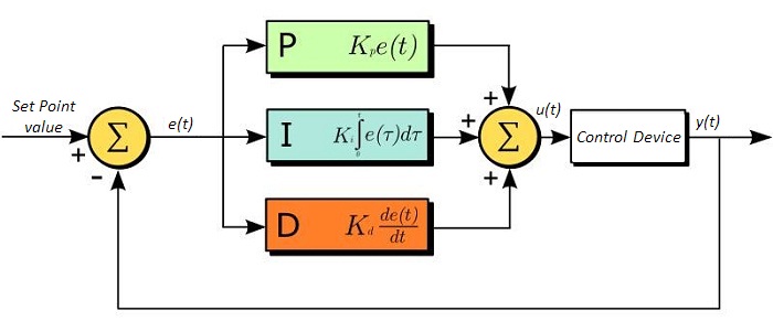
The PID circuit is often utilized as a control loop feedback controller and is commonly used for many forms of servo circuits. The letters making up the acronym PID correspond to Proportional (P), Integral (I), and Derivative (D), which represents the three control settings of a PID circuit. The purpose of any servo circuit is to hold the system at a predetermined value (set point) for long periods of time. The PID circuit actively controls the system so as to hold it at the set point by generating an error signal that is essentially the difference between the set point and the current value. The three controls relate to the time-dependent error signal. At its simplest, this can be thought of as follows: Proportional is dependent upon the present error, Integral is dependent upon the accumulation of past error, and Derivative is the prediction of future error. The results of each of the controls are then fed into a weighted sum, which then adjusts the output of the circuit, u(t). This output is fed into a control device, its value is fed back into the circuit, and the process is allowed to actively stabilize the circuit’s output to reach and hold at the set point value. The block diagram below illustrates the action of a PID circuit. One or more of the controls can be utilized in any servo circuit depending on system demand and requirement (i.e., P, I, PI, PD, or PID).
Through proper setting of the controls in a PID circuit, relatively quick response with minimal overshoot (passing the set point value) and ringing (oscillation about the set point value) can be achieved. Let’s take as an example a temperature servo, such as that for temperature stabilization of a laser diode. The PID circuit will ultimately servo the current to a Thermo Electric Cooler (TEC) (often times through control of the gate voltage on an FET). Under this example, the current is referred to as the Manipulated Variable (MV). A thermistor is used to monitor the temperature of the laser diode, and the voltage over the thermistor is used as the Process Variable (PV). The Set Point (SP) voltage is set to correspond to the desired temperature. The error signal, e(t), is then the difference between the SP and PV. A PID controller will generate the error signal and then change the MV to reach the desired result. For example, if e(t) states that the laser diode is too hot, the circuit will allow more current to flow through the TEC (proportional control). Since proportional control is proportional to e(t), it may not cool the laser diode quickly enough. In that event, the circuit will further increase the amount of current through the TEC (integral control) by looking at the previous errors and adjusting the output to reach the desired value. As the SP is reached (e(t) approaches zero), the circuit will decrease the current through the TEC in anticipation of reaching the SP (derivative control).
Please note that a PID circuit will not guarantee optimal control. Improper setting of the PID controls can cause the circuit to oscillate significantly and lead to instability in control. It is up to the user to properly adjust the PID gains to ensure proper performance.
PID Theory
The output of the PID control circuit, u(t), is given as
where
Kp= Proportional Gain
Ki = Integral Gain
Kd = Derivative Gain
e(t) = SP - PV(t)
From here we can define the control units through their mathematical definition and discuss each in a little more detail. Proportional control is proportional to the error signal; as such, it is a direct response to the error signal generated by the circuit:
Larger proportional gain results in larger changes in response to the error, and thus affects the speed at which the controller can respond to changes in the system. While a high proportional gain can cause a circuit to respond swiftly, too high a value can cause oscillations about the SP value. Too low a value and the circuit cannot efficiently respond to changes in the system.
Integral control goes a step further than proportional gain, as it is proportional to not just the magnitude of the error signal but also the duration of the error.
Integral control is highly effective at increasing the response time of a circuit along with eliminating the steady-state error associated with purely proportional control. In essence integral control sums over the previous error, which was not corrected, and then multiplies that error by Ki to produce the integral response. Thus, for even small sustained error, a large aggregated integral response can be realized. However, due to the fast response of integral control, high gain values can cause significant overshoot of the SP value and lead to oscillation and instability. Too low, and the circuit will be significantly slower in responding to changes in the system.
Derivative control attempts to reduce the overshoot and ringing potential from proportional and integral control. It determines how quickly the circuit is changing over time (by looking at the derivative of the error signal) and multiplies it by Kd to produce the derivative response.
Unlike proportional and integral control, derivative control will slow the response of the circuit. In doing so, it is able to partially compensate for the overshoot as well as damp out any oscillations caused by integral and proportional control. High gain values cause the circuit to respond very slowly and can leave one susceptible to noise and high frequency oscillation (as the circuit becomes too slow to respond quickly). Too low and the circuit is prone to overshooting the SP value. However, in some cases overshooting the SP value by any significant amount must be avoided and thus a higher derivative gain (along with lower proportional gain) can be used. The chart below explains the effects of increasing the gain of any one of the parameters independently.
| Parameter Increased | Rise Time | Overshoot | Settling Time | Steady-State Error | Stability |
|---|---|---|---|---|---|
| Kp | Decrease | Increase | Small Change | Decrease | Degrade |
| Ki | Decrease | Increase | Increase | Decrease Significantly | Degrade |
| Kd | Minor Decrease | Minor Decrease | Minor Decrease | No Effect | Improve (for small Kd) |
Tuning
In general the gains of P, I, and D will need to be adjusted by the user in order to best servo the system. While there is not a static set of rules for what the values should be for any specific system, following the general procedures should help in tuning a circuit to match one’s system and environment. A PID circuit will typically overshoot the SP value slightly and then quickly damp out to reach the SP value.
Manual tuning of the gain settings is the simplest method for setting the PID controls. However, this procedure is done actively (the PID controller turned on and properly attached to the system) and requires some amount of experience to fully integrate. To tune your PID controller manually, first the integral and derivative gains are set to zero. Increase the proportional gain until you observe oscillation in the output. Your proportional gain should then be set to roughly half this value. After the proportional gain is set, increase the integral gain until any offset is corrected for on a time scale appropriate for your system. If you increase this gain too much, you will observe significant overshoot of the SP value and instability in the circuit. Once the integral gain is set, the derivative gain can then be increased. Derivative gain will reduce overshoot and damp the system quickly to the SP value. If you increase the derivative gain too much, you will see large overshoot (due to the circuit being too slow to respond). By playing with the gain settings, you can maximize the performance of your PID circuit, resulting in a circuit that quickly responds to changes in the system and effectively damps out oscillation about the SP value.
| Control Type | Kp | Ki | Kd |
|---|---|---|---|
| P | 0.50 Ku | - | - |
| PI | 0.45 Ku | 1.2 Kp/Pu | - |
| PID | 0.60 Ku | 2 Kp/Pu | KpPu/8 |
While manual tuning can be very effective at setting a PID circuit for your specific system, it does require some amount of experience and understanding of PID circuits and response. The Ziegler-Nichols method for PID tuning offers a bit more structured guide to setting PID values. Again, you’ll want to set the integral and derivative gain to zero. Increase the proportional gain until the circuit starts to oscillate. We will call this gain level Ku. The oscillation will have a period of Pu. Gains for various control circuits are then given below in the chart.
| Posted Comments: | |
| No Comments Posted |