Pulse Distortion: Preserving Rectangular Pulse Shapes

Click to Enlarge

Figure 1: An extreme example of pulse distortion. Due to slow system response, the output pulse is a distorted version of the input pulse.

Click above to download the full report.

What 3 dB system bandwidth is required for rectangular output pulses?

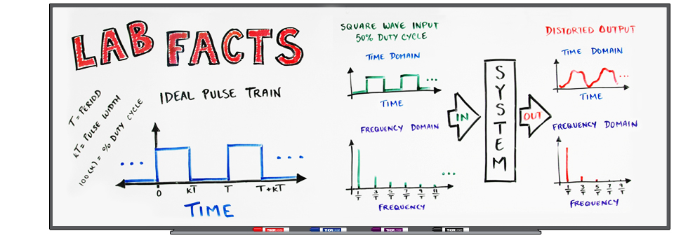
Pulse distortion is deformation of the ideal pulse profile, and it occurs in output signals when the system cannot respond as fast as the amplitude of the input signal changes. Distortion of pulses output by a system is expected when the bandwidth of the system is not sufficient to accommodate the bandwidth of the input signal. This effect is frequently seen when the input signal is a square wave or rectangular pulse train with a high repetition rate. The distorted rectangular pulse will often have a rounded appearance, as illustrated in Figure 1.

Pulse distortion can be a concern for any system intended to output a scaled version of an input signal. An example is a system that includes a laser diode driver that accepts an input signal from a function generator and supplies a current signal to a laser diode. The driver is expected to output a current signal that is a good representation of the input signal supplied by the function generator. Systems are typically designed to minimize the distortion in the output signal when the input signal frequencies are within the system's specified bandwidth, which is a frequency range over which the system's response is optimal.

It is not always possible, or desirable, to use a system whose response is fast enough to provide an undistorted output pulse. When the bandwidth of the input signal is greater than the system's 3 dB bandwidth, the output signal can be expected to exhibit the effects of pulse distortion.

In this Lab Fact, different broadband, periodic rectangular pulse trains were input to a laser-based system with a 3 dB cutoff frequency of 750 kHz. The distortion in the resulting output signals were analyzed using two approaches. One considered the frequency content of the input and output signals. The other method compared the shapes of the input and output pulses. These approaches were used to:

• Investigate the pulse distortion in the output signals when different rectangular pulse trains were used as input signals.
• Investigate the pulse quality that results from applying the 9X rule relating 3 dB system cutoff frequency and the input signal repetition rate.
• Develop an approach for numerically rating the pulse shape of nominally rectangular output pulse profiles.

What is a rectangular pulse train? 

Click to Enlarge

Figure 2: An ideal rectangular pulse train as a function of time (t). The period (T), duty cycle (κ), and high-state amplitude (X) are labeled.

Input Rectangular Pulse Trains
Rectangular pulse trains are signals consisting of a repeating rectangular pulse, which looks like a top hat and is produced when the signal's amplitude transitions from a minimum to a maximum value, dwells at the maximum value for some time, and then transitions back to the minimum value. This is illustrated in Figure 2.

For ideal rectangular pulses, the signal requires no time to switch between the two amplitudes, so the transition is instantaneous. The rectangular pulse repeats after a constant amount of time called a period (T). The pulse width is the length of time the pulse spends at the high value, and the fractional duty cycle (κ) is the fraction of time the pulse remains in the high state. Rectangular pulse trains can have any duty cycle between 0 and 1, which can be calculated by dividing the pulse width by the period. The duty cycle is frequently expressed as a percentage of the period. In the figure, the maximum amplitude, or high state, amplitude is equal to X, and the minimum, or low state amplitude, is equal to 0.

If the waveform in Figure 2 were plotted as a function of frequency, the frequency axis would extend to infinity. An infinite number of frequencies are required to create an ideal rectangular pulse, since high frequencies are required to generate infinitely short transitions. In general, a periodic signal with sharp and narrow features requires many high frequencies above its fundamental frequency, which is equal to the reciprocal of the period.

Return to Top

1

Why does a system's 3 dB cutoff frequency matter? 

Consequences of Limited System Bandwidth
The bandwidth of a system is a measure of how quickly the system can respond to changes in the input signal or, equivalently, it is an indication of the highest frequency the system can support. It is not unusual for the system bandwidth to be smaller than the bandwidth of the input signal. When this mismatch occurs, the higher frequency components of the input signal will not be preserved in the output signal, resulting in pulse distortion.

If the higher frequency components are stripped from a rectangular pulse train, the sharp corners of the pulses will become rounded, and the minimum time required to transition between the low and high amplitude states will lengthen. If enough high frequency components are removed, the input rectangular pulse train can be transformed into a sine wave.

3 dB Cutoff Frequency
The bandwidth of a system is often described by its 3 dB bandwidth, instead of the absolute maximum range of frequencies over which it provides some response. The 3 dB bandwidth is commonly specified since the maximum frequency range can be difficult to determine, and since frequencies outside the 3 dB bandwidth usually contribute minimally to the system's performance. It is often convenient to think of the output signal consisting of only the input signal components with frequencies below the 3 dB cutoff frequency, since the system strongly attenuates frequencies higher than the 3 dB cutoff. However, frequencies above the 3 dB cutoff can still contribute to the output signal. The 3 dB cutoff frequency is recommended for use as a general reference for estimating how the frequency content of the output and input signals can be expected to differ.

Return to Top

2

Experimental Setup

Experimental Setup
The experimental setup is pictured at the top of this page. Rectangular pulse trains from a function generator were input to a CLD1010LP Mount and Current and Temperature Controller for a Fiber-Pigtailed Laser Diode. The output current provided by the controller, which included a user-specified constant current component, was input to a fiber-pigtailed laser diode mounted in the controller. The magnitude of the constant current component was chosen so that the total current sent to the laser diode always exceeded its lasing threshold current. The modulated input current from the driver resulted in the laser diode emitting a modulated optical signal.

The optical signal was incident upon a DET02AFC 1 GHz FC/PC-Coupled Photodetector, which was connected to an 80 MHz function generator. The 3 dB cutoff frequency of the system was determined to be 750 kHz using the procedure described in the full report. The rectangular pulse trains from the function generator were compared with the detected optical signals by analyzing both the frequency content of the signals and the shapes of the waveforms' pulses.

Return to Top

3

How does changing the rep rate affect pulse distortion?

Click to Enlarge

Figure 3: These output waveforms^† were measured for square wave input signals with rep rates approaching the 3 dB cutoff frequency of 750 kHz. This frequency was nine times greater than the 83.3 kHz rep rate signal (dark red), which resulted in the output waveform being a reasonable representation of the input square wave.

^†The overshoot on the rising edges and undershoot on the falling edges of the pulses are artifacts, likely from an impedance mismatch between components in the system.

Increasing the Repetition Rate of the Input Square Wave
Square waves are rectangular pulse trains with 50% duty cycles. Square waves always have pulse widths^* equal to half the duration of the period. However, the absolute length of the period can be controlled by varying the repetition rate (rep rate). The rep rate is the reciprocal of the period.

Square waves with different rep rates were input to the system described above. The measured output pulses, some of which are plotted in Figure 3, show how pulse distortion increased as the rep rate approached the 3 dB cutoff frequency.

As the rep rate increased, the pulse duration decreased, but the time the output signal needed to transition between the low and high amplitude states did not change. The result was that as the rep rate increased, the fraction of the period the signal needed to transition between the low and high amplitude states increased, resulting in the sides of the pulses sloping farther away from vertical. The top of the pulse also became less flat with increasing rep rate. For the extreme case when the rep rate was equal to the 3 dB bandwidth, the output signal resembled a sine wave.

A useful tool for exploring the relationship between the 3 dB cutoff frequency and the rep rate is the Fourier series expansion of an ideal square wave,

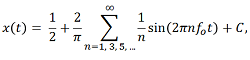
which shows that the square wave can be represented as the sum of an infinite number of sine waves. The constant (C) shifts the average amplitude of the square wave but does not affect the pulse shape. The rep rate of the input signal is equal to the frequency of the 1^st order expansion term (n = 1). This frequency is also called the fundamental frequency (_o). The higher-order frequency components in the square wave have frequencies that are odd-integer-multiples (n = 3, 5, ...) of the fundamental frequency.

Keeping this expansion in mind while considering the measurement results reveals a couple of interesting things:

• Increasing the rep rate increases the frequency of each term.
• The 1^st order expansion term (n = 1) is the sinusoid with the largest amplitude.

During the experiment, as the rep rate increased, fewer input signal components had frequencies below the 3 dB cutoff frequency. Pulse distortion in the output signal was caused by signal components with frequencies above this threshold being strongly attenuated. The output waveform began to more closely resemble a sine wave, since fewer and fewer terms had frequencies below the 3 dB cutoff frequency. This allowed the 1^st order sine wave term to begin to dominate. When the rep rate matched the 3 dB frequency, only the 1^st order term had a frequency below the 3 dB cutoff frequency.

^*The time the signal spends in the high-amplitude state.

Return to Top

4

How does the duty cycle affect the pulse shape and required system bandwidth?

Click to Enlarge

Figure 4: The plotted output waveforms resulted from periodic rectangular pulse trains with 20% duty cycles input with the indicated rep rates. The detrimental effect on pulse shape resulting from reducing the duty cycle while maintaining the rep rate can be seen by comparing the 83.3 kHz case plotted above with that plotted in Figure 3.

Reducing the Duty Cycle of the Input Rectangular Pulse Train
If the rep rate of the input rectangular pulse train is held constant, reducing its duty cycle decreases the pulse width^*. Reducing the pulse width while keeping the rep rate constant will increase the pulse distortion in the output signal, if the system bandwidth is smaller than the signal bandwidth. The pulse distortion worsens due to the transition time between the low- and high-state amplitudes becoming a larger fraction of the pulse width. Another consequence is that the signal has less time to stabilize at the high-state amplitude before transitioning to the low-state amplitude.

Figure 4 shows a selection of pulses measured at the output of the experimental system when the input signal had a duty cycle of 20%. The pulse profile was recognizably rectangular for a rep rate of 83.3 kHz, when the system bandwidth was approximately nine times the system bandwidth. When the rep rate was 200 kHz, the system bandwidth was over three times the rep rate, but the output pulse had a sinusoidal shape. This is different than for the 50% duty cycle case, in which an even higher rep rate of 250 kHz resulted in a pulse with a recognizably rectangular profile.

^*The time the signal spends in the high-amplitude state.

Return to Top

6

How do the duty cycles of the input and output signals compare?

Click to Enlarge

Figure 5: Duty cycles of input and output pulse trains differed as the rep rate approached the 750 kHz system bandwidth. As the higher order frequency components were attenuated, the output signal duty cycle approached 50%.

Duty Cycles of the Input and Output Pulse Trains
Increasing the rep rate of an input signal whose duty cycle is not 50% can both cause output pulse distortion and result in an output signal whose duty cycle is closer to 50% than expected. Measurements showing this trend for the 750 kHz system described previously are plotted in Figure 5. For rep rates up to between 200 and 300 kHz, the duty cycles of the input and output signals agreed well. The duty cycles of the output and input duty cycles began to differ when the system's bandwidth was between three or four times the rep rate. For higher rep rates, the duty cycle of the output signal began to converge to 50%.

This effect occurs due to the fundamental frequency component of the input signal being a sine wave. Sine waves have 50% duty cycles, and the higher frequency components are needed to shape the waveform into one with the desired duty cycle. Increasing the rep rate results in more input signal components having frequencies higher than the system's 3 dB cutoff frequency. Since these higher frequency components are highly attenuated by the system, the output signal becomes dominated by the fundamental frequency component.

Return to Top

7

What is a way to numerically rate pulse distortion?

Click to Enlarge

Figure 6: A square wave (green) and a sinusoid (blue), both have pulse widths equal to 0.5T. The dashed segments show the transitions from the low to the high signal states. For the square wave, the transition is infinitely short and the dwell time at each state is equal to 0.5T. The exact opposite is true for the sinusoid.

Quality Factor Definition
The quality factor approach was developed to predict and assess the pulse distortion of nominally rectangular output pulses. It is a way to visualize the principle of Fourier analysis, without the need of performing Fourier transforms, working with Fourier series, or conducting similar analysis. This method rates the similarity of a measured pulse profile to an ideal rectangular pulse profile. It does this by comparing the rise time of the measured pulse with the width of the ideal pulse it approximates.

Figure 6 shows a period of an ideal square wave pulse in green and a period of the 1^st order term of its Fourier series expansion, a sine wave, in blue. The dashed lines show their rising edges. A maximum quality factor of one describes pulses with ideal rectangular profiles, which require no time to transition between min and max amplitudes. Pulses with zero quality factors have transition times that are as long as the ideal pulse is wide. For example, the blue pulse in Figure 6 has a zero quality factor, since its 0.5T transition time equals the width of the ideal pulse.

Signal noise and instability can make it difficult to accurately measure the full transition time for real signals. Instead, a measurement is typically made of the time needed to transition from a point slightly above the minimum amplitude to another point slightly below the maximum amplitude. It is common to locate these alternate points at amplitudes 10% and 90% up the rising edge. The quality factor (Γ) is calculated using this measurement of the pulse's rise time (_r), as well as the width of the ideal rectangular pulse (W),

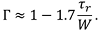
A more complete discussion of how this approximation was derived and why use is not recommended for duty cycles ≥50% is provided in the full report. 

Return to Top

8

How does the duty cycle of the input signal affect the range of quality factors?

Click to Enlarge

Figure 7: Periodic rectangular pulse trains were input to a system with a 3 dB cutoff frequency of 750 kHz, and quality factors^* of the output waveforms were computed. The two curves for the 80% case correspond to quality factors computed using the ideal high and low state widths. The lines connecting the data points are guides for the eye.

^* Curves are labeled with the word "High" or "Low" to indicate that quality factor values were calculated using the high-state or low-state, respectively, widths of the ideal rectangular pulses.

Quality Factor Measurements
The blue curve in Figure 7 plots the quality factors calculated for the output pulses when the input waveforms had 50% duty cycles and repetition rates between 25 kHz and 750 kHz. The quality factor computed for the 83.3 kHz rep rate case was 0.87, which compares well with the maximum possible quality factor of one. The high quality factor computed for the 83.3 kHz case supports the use of the 9X rule, which refers to the minimum recommended ratio between the 3 dB cutoff frequency and the rep rate of the input rectangular pulse train.

The 0.58 quality factor computed for the 250 kHz, 50% duty cycle case supports the qualitative observation that despite some pulse distortion in the output signal, the pulse profile was more rectangular than sinusoidal. This was the case even though only two signal components from the input signal had frequencies within the 750 kHz system bandwidth. When the rep rate was 750 kHz, the output waveform appeared sinusoidal and the quality factor was zero.

Quality factors for the 20% duty cycle case are plotted in red. The 0.68 quality factor for an 83.3 kHz rep rate corresponded to an identifiably rectangular pulse profile. However, there was more pulse distortion than for the 83.3 kHz rep rate case with the 50% duty cycle, in which the pulse had a quality factor of 0.87. This illustrates that reducing the duty cycle, while maintaining the rep rate results in increased output pulse distortion. To obtain a 0.87 quality factor, the rep rate of the 20% duty cycle waveform would have to be lowered to approximately 33 kHz.

When the rep rate of the 20% duty cycle waveform was increased to approximately 250 kHz, the quality factor became zero. Quality factors corresponding to higher repetition rates were negative. Physically, this means that the rise time was longer than input pulse width. Under these conditions, it can be challenging to accurately measure rise time.

The green (80% High) curve demonstrates that when the duty cycle of the input signal is >50%, the minimum quality factor is positive. Since the scale does not extend to zero, it is difficult to compare these quality factors with other duty cycle cases. In addition, the quality factor rates the shape of the pulse, but not the low-state segments of the output waveform, which are more significantly distorted. To address these concerns, the quality factor can instead be computed using the low-state widths. These alternate 80% data were plotted in gold and resembled the 20% duty cycle data, as expected.

The quality factors plotted in Figure 7 concisely show the influence of pulse width, repetition rate, and input duty cycle on the distortion of the output pulse. When other parameters are held constant, output signal distortion increases when:

• Rep rate is increased.
• Duty cycle is decreased.
• System bandwidth is decreased.

Return to Top

9