 Products Home / Optical Elements / Test Targets, Calibration Targets, and Reticles / Slant Edge MTF Target
Slant Edge MTF Target
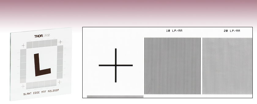
- Slant Edge Test Target Evaluates Spatial Frequency Response of Imaging System
- L-Shaped, 5° Slanted Edge and Ronchi Rulings on 2" x 2" Plate
- Four Cross Patterns for Alignment
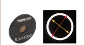
R2L2S2P
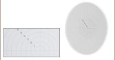
Enlarged View of 10 lp/mm and 20 lp/mm Ronchi Rulings and Cross Pattern on R2L2S2P


Please Wait
| Specifications | |
|---|---|
| Design | LRa Chrome-on-Glass |
| Substrate | Soda Lime Glass |
| Chrome Thickness | 0.120 µm |
| Chrome Optical Density | OD ≥3.0 at 430 nm |
| Substrate Thickness | 0.06" (1.5 mm) |
| Surface Flatness | ≤15 µm |
| Line Spacing Toleranceb | ±1 µm |
| Line Width Toleranceb | ±0.5 µm |
Click to Enlarge
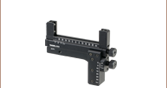
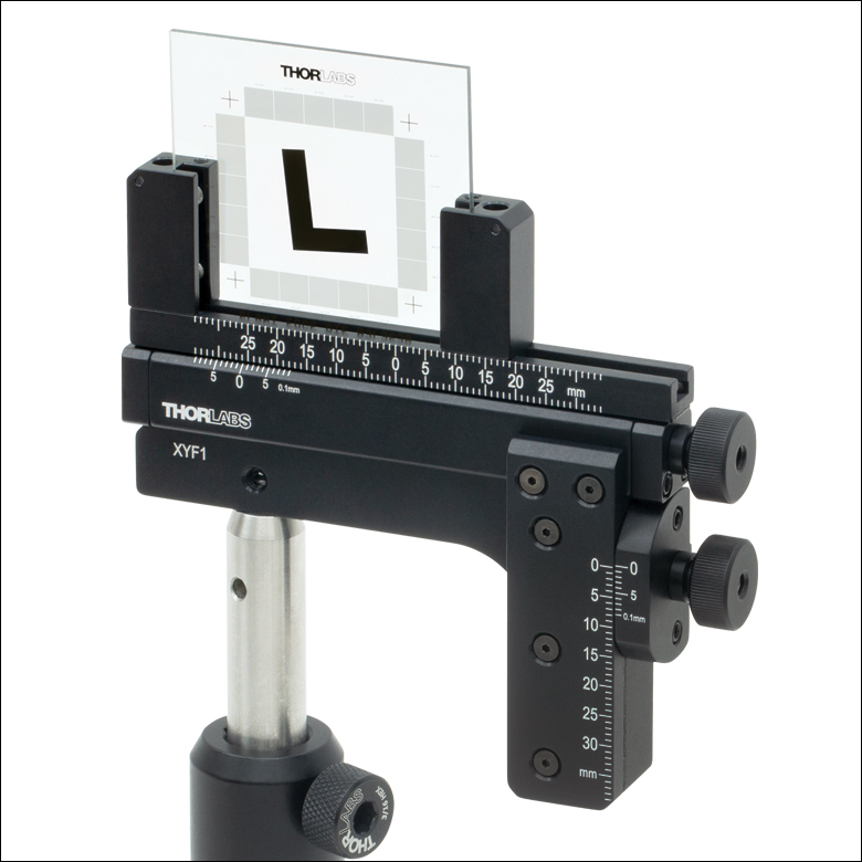
Figure 1.1 An R2L2S2P Slant Edge MTF Target Mounted in an XYF1 Test Target Positioner
Features
- Determine Modular Transfer Function (MTF) of an Imaging System
- 5° Slanted, L-Shaped Pattern (ISO 12233 Compatible)
- 20 Variable Ronchi Rulings, 10 lp/mm to 200 lp/mm
Thorlabs' Slant Edge MTF Target allows the user to determine the spatial frequency response of an imaging system via a slant edge pattern or Ronchi rulings. The slant edge pattern is L-shaped and tilted at 5° for compatibility with ISO 12233. The Ronchi rulings include twenty individual rulings, each 5 mm x 5 mm in dimension and ranging in resolution from 10 line pairs per millimeter (lp/mm) to 200 lp/mm in 10 lp/mm intervals. Made from a soda lime glass substrate with low-reflectivity, vacuum-sputtered chrome, the target also features a cross pattern at each of the four corners of the overall pattern for alignment. Each pattern is manufactured using photolithography, allowing for edge features to be resolved down to approximately 1 µm. The high edge sharpness provided by this method is essential when using the modulation transfer function (MTF), described below, to determine the performance of an imaging system.
Mounting
To mount this target, Thorlabs offers the XYF1(/M) Test Target Positioning Mount (see Figure 1.1). This mount is capable of translating the target over a 50 mm (1.97") x 30 mm (1.18") area and secures the target using nylon-tipped setscrews. The mount contains five 8-32 (M4) taps for six post-mountable orientations.
Modulation Transfer Function
The modulation transfer function (MTF) is used to determine the resolution and performance of an imaging system. Several kinds of targets exist to measure the MTF of a system, including sine wave targets, grill targets, and the slanted edge targets discussed here. For the slant edge method, a slant edge target, such as the one featured on this page, is imaged. The target consists of a distinct dark edge that is tilted at some angle, usually between one and five degrees. The edge should be produced using a method that will produce as distinct an edge as possible. In the case of the target sold here, photolithography is used.
To calculate the MTF, begin with the edge spread function (ESF), which is the intensity of the image as a function of spatial position as the the edge is approached and crossed over (see Zhang et al., Proc. SPIE 8293, 2012). Due to imperfections in the imaging system, the ESF will be sloped on the border of the slanted edge, as opposed to being a perfect step function. Next, take the derivative of the ESF to produce the line spread function (LSF). Finally, take the Fourier transform of the LSF and normalize it to produce the MTF. The MTF, which will range from zero to one, can be plotted versus frequency (typically measured in cycles/mm). Frequencies with a corresponding MTF value close to one will be reproduced at approximately their original resolution. As the frequency increases, the MTF will fall to zero and the frequency will become indiscernible. The frequency that corresponds to a MTF of 0.5 is typically used as a benchmark to compare different imaging systems.
Various packages are available commercially for the calculation of the MTF using MATLAB® or ImageJ. One such package for MATLAB can be found here, while a package for ImageJ can be found here.
| Targets Selection Guide | ||||
|---|---|---|---|---|
| Resolution Test Targets | Calibration Targets | Distortion Test Targets | Slant Edge MTF Target | Stage Micrometers |

Jason Williamson
Director of Business Development
Thorlabs Spectral Works
Need a Quote?
| Customization Parameters | ||
|---|---|---|
| Substrate Sizea | Min | 8 mm x 8 mm (5/16" x 5/16") |
| Max | 85 mm x 85 mm (3.35" x 3.35") | |
| Substrate Materials | Soda Lime Glass UV Fused Silica Quartz |
|
| Coating Material | Chromeb Low-Reflectivity Chromec |
|
| Coating Optical Density | ≥3d or ≥6e @ 430 nm | |
| Minimum Pinhole/Spot | Ø1 µm | |
| Minimum Line Width | 1 µm | |
| Line Width Tolerance | -0.25 / +0.50 µm | |
| Maximum Line Density | 500 lp/mm | |
Custom OEM Test Targets and Reticles
Our in-house photolithographic design and production capabilities enable us to create a range of patterned optics. We manufacture test targets, distortion grids, and reticles at our Thorlabs Spectral Works facility in Columbia, South Carolina. These components have served a wide variety of applications, being implemented in microscopes, imaging systems, and optical alignment setups.
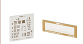
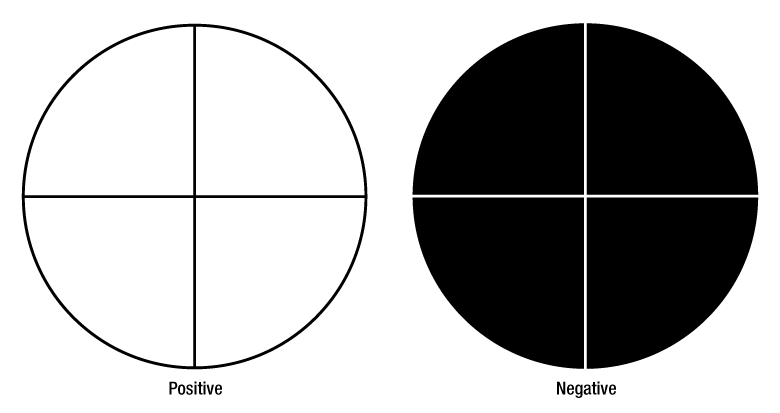
In addition to our catalog test targets and reticles offered from stock, we can provide custom chrome patterns on soda lime, UV fused silica, or quartz substrates from 8 mm by 8 mm up to 85 mm by 85 mm. Substrates can be cut to shape for your application. Our photolithographic coating process allows us to create chrome features down to 1 µm. A few sample patterns are shown below, which can be made positive or negative, as shown in the image directly below.
For a quote on custom test targets and reticles, please contact us at TSW@thorlabs.com.
Sample Patterns
 Click to Enlarge
 Click to Enlarge
 Click to Enlarge
 Click to Enlarge
 Click to Enlarge
 Click to Enlarge
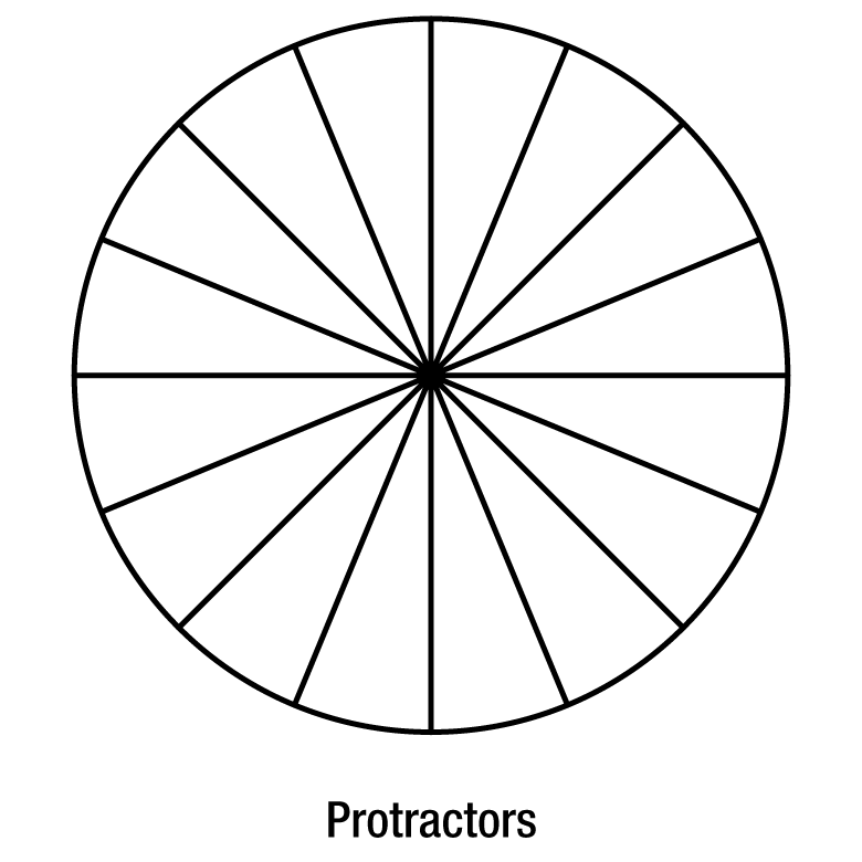 Click to Enlarge
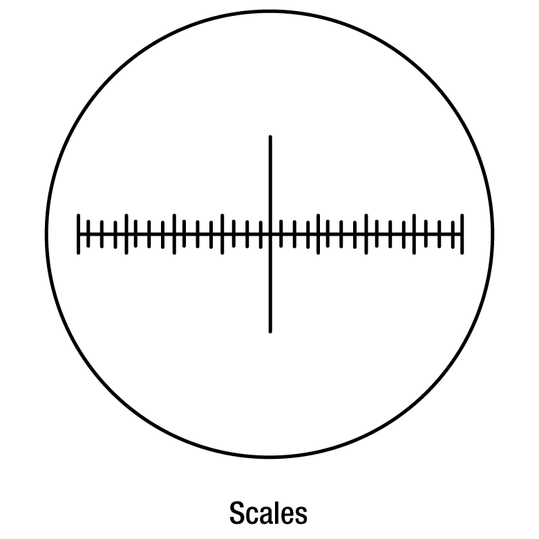 Click to Enlarge
Example Applications
- Etched Reticles
- Gray Scale Masks
- Resolution Reticles
- Diagnostic Reticles
- Recreational Scopes
- Notching Reticles
- Eyepiece Scales
- Illuminated Crosshairs
- Obstruction Targets
- Binocular Reticles
Click to Enlarge
Positive and Negative Crosshair Sample Pattern
This tab details an optimal cleaning technique developed by our engineers for cleaning reticles, test targets, distortion targets, and calibration targets.
Cleaning Procedure
- Use a clean wet sponge, preferably made of polyvinyl alcohol (PVA), and dish detergent to gently scrub the front and back surfaces of your reticle or target.
- Rinse with water.
- Blow dry with clean dry air, or allow the reticle or target to air dry on a clean surface.
We do not suggest using a towel, rag, or wipe to dry the surface. If contamination persists, soak the reticle or target in a detergent and water solution for 1 hour, repeating as necessary.
| Posted Comments: | |
Yiğit Can Acar
(posted 2023-05-05 04:04:39.673) Dear Official,
I am writing this e-mail from “YUBA Teknoloji”, an optics company in Ankara, Turkey. I am also working as electrical engineer in this firm. In our company, we would like to build an MTF test system with a slanted edge target and off axis parabolic mirror. In your website, i examined your L shaped 5 degree slanted edge MTF target (https://www.thorlabs.com/newgrouppage9.cfm?objectgroup_id=7500) and found that this component can be useful for us. However, i have some important questions. First of all, is it avaible to conduct an experiment in visible and near infrared (VIS and NIR) spectrum with this Slant Edge MTF Target ? Since we are planning to illuminate this target from the front, we are going to need a well transparent material in our experiment and we need to know its transmission characteristics. In addition, which type of light source is compatible with this target ? We also would like to order additional mechanical components like XYF1 mount and other holders and post holders. Is it possible for you to come up with a complete suitable set and quotation proposal including Slant Edge Target, XYF1 mount and holders ?
Yours Sincerely,
Yiğit Can Acar. ksosnowski
(posted 2023-05-11 09:45:06.0) Hello, thanks for reaching out to Thorlabs. R2L2S2P uses our soda lime substrate, for which the data can be found on our main Resolution Target page (e.g. see R1DS1P). This maintains transmission throughout VIS and NIR ranges, and while we do not have a single light source for all scenarios, we have a variety of broadband lamps like SLS201 which you may consider for this range. I have reached out directly to discuss this application in further detail. Our sales team can also be reached directly via sales@thorlabs.com for a quote. ksosnowski
(posted 2023-05-11 09:45:06.0) Hello, thanks for reaching out to Thorlabs. R2L2S2P uses our soda lime substrate, for which the data can be found on our main Resolution Target page (e.g. see R1DS1P). This maintains transmission throughout VIS and NIR ranges, and while we do not have a single light source for all scenarios, we have a variety of broadband lamps like SLS201 which you may consider for this range. I have reached out directly to discuss this application in further detail. Our sales team can also be reached directly via sales@thorlabs.com for a quote. Martin Bordenave
(posted 2020-01-07 09:07:12.863) Dear Sir or Madam,
My name is Martin Diego Bordenave, I work as an optical engineering at Satellogic, an Argentinean, earth-observation company.
I would like to know is it is possible to buy a Slant Edge MTF Target similar to the R2L2S2P but instead of using a square substrate using a circular substrate of 2" diameter.
I look forward to hearing from you.
Best regards,
Dr. Martín Diego Bordenave
Telephone: +54 11 5219 0100
e-mail: martin.bordenave@satellogic.com YLohia
(posted 2020-01-07 12:33:17.0) Hello Martin, thank you for contacting Thorlabs. Custom items can be requested by emailing us at techsupport@thorlabs.com. I will reach out to you directly to discuss the possibility of offering this custom item. Ralf Noijen
(posted 2019-06-07 04:18:21.85) Dear Thorlabs,
I have two comments. My colleague had ordered the target which we received today. I inspected it under a microscope and found quite some damages, is that normal?
Secondly I found a link to a mtf measurement application for imageJ which is not working.
Can you please help.
BR
Ralf YLohia
(posted 2019-06-07 10:56:56.0) Hello Ralf, thank you for contacting Thorlabs. We are sorry to hear about the damaged item. This is certainly not normal -- I am reaching out to you directly to look into what sort of defects your piece has. Please use this link for the ImageJ package: https://imagej.nih.gov/ij/plugins/se-mtf/index.html. It is a non-Thorlabs website and it is working for on our end. dmiles
(posted 2017-01-09 13:36:40.047) The Slant Edge MTF Target looks very useful to us. It would help a lot if there were a scale image of it at normal incidence so we could design with the corner of the "L" at the focus of our system before we receive it. We are in a time crunch and our designer would be helped by that information. tfrisch
(posted 2017-01-10 09:37:29.0) Hello, thank you for contacting Thorlabs. we do have a CAD drawing that may be useful for your application. It can be found by clicking the documents icon below. I will send you a link directly as well. sebastien.avila
(posted 2015-01-07 12:08:20.28) Hello,
I would like to know if the clear parts of the target R2L2S2P are transparent or opaque white? Is it meant to be backlighted?
Should I use a diffuse source or a collimated source?
Thank you very much.
Sébastien AVILA
R&D VISION- France besembeson
(posted 2015-01-19 01:12:36.0) Response from Bweh at Thorlabs: The substrate is made from soda lime so transmission properties will be like that for soda lime in areas without the chrome. R2L2S2P is a positive target designed for front-lit applications. For MTF determination, you would typically image the slanted "L" so diffused or large diameter collimated source should be okay. |