 Products Home / Optical Elements / Optical Lenses / Spherical Singlet Lenses / Plano-Concave Spherical Lenses / N-BK7 Plano-Concave Spherical Lenses / N-BK7 Plano-Concave Lenses, AR Coating 350 - 700 nm
N-BK7 Plano-Concave Lenses, AR Coating 350 - 700 nm
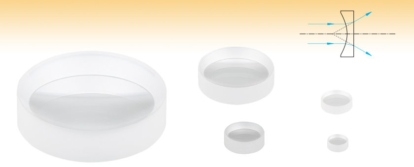
- Negative Focal Length Used to Diverge Collimated Beams
- AR Coated for the 350 - 700 nm Range
- Zemax Files Available
LC1315-A
(Ø2")
LC1715-A
(Ø1")
LC1054-A
(Ø1/2")
LC1906-A
(Ø9 mm)
LC1975-A
(Ø6 mm)


Please Wait
| Common Specifications | |
|---|---|
| Lens Shape | Plano-Concave |
| Substrate Material | N-BK7 (Grade A)a |
| AR Coating Range | 350 - 700 nm |
| AR Coating Reflectance | Ravg < 0.5% per Surface |
| Diameters Available | 6 mm, 9 mm, 1/2", 25 mm, 1", or 2" |
| Diameter Tolerance | +0.0/-0.1 mm |
| Thickness Tolerance | ±0.1 mm |
| Focal Length Tolerance | ±1% |
| Design Wavelength | 587.6 nm (Except Ø25 mm Lenses) 632.8 nm (Ø25 mm Lenses) |
| Index of Refraction @ 633 nm |
1.515 |
| Surface Quality | 40-20 Scratch-Dig |
| Surface Flatness (Plano Side) |
λ/2 |
| Spherical Surface Powerb (Concave Side) |
3λ/2 |
| Surface Irregularity (Peak to Valley) |
λ/4 |
| Damage Thresholdc | 7.5 J/cm2 (532 nm, 10 ns, 10 Hz, Ø0.504 mm) |
| Abbe Number | vd = 64.17 |
| Centration | <3 arcmin |
| Clear Aperture | >90% of Diameter |
 Zemax Files Zemax Files |
|---|
| Click on the red Document icon next to the item numbers below to access the Zemax file download. Our entire Zemax Catalog is also available. |
Features
- Material: N-BK7
- AR Coated for the 350 - 700 nm Range
- Choose from 6 Diameters: Ø6 mm, Ø9 mm, Ø1/2" (Ø12.7 mm), Ø25 mm, Ø1" (Ø25.4 mm), or Ø2" (Ø50.8 mm)
- Offers Excellent Transmission Throughout the Visible and Near Infrared
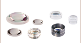
These Plano-Concave lenses, which are fabricated from RoHS-compliant N-BK7 glass, have a broadband antireflection coating for the 350 - 700 nm range. This coating greatly reduces the 4% losses per surface incurred when using an uncoated lens (see the Graphs tab for details).
N-BK7 is one of the most common optical types of glass used for high quality optical components. It is typically chosen whenever the additional benefits of UV fused silica (i.e., good transmission further into the UV and a lower coefficient of thermal expansion) are not necessary. However, for particularly harsh environments where the optic will be exposed to alkalis and acids, consider our N-SF11 plano-concave lenses. Since the Abbe Number of N-SF11 (25.76) is lower than that for N-BK7 (64.17), lenses fabricated from N-SF11 will exhibit higher dispersion than those fabricated from N-BK7.
Like all plano-concave lenses, these lenses have negative focal lengths and can be used to diverge collimated beams. In this case, the curved surface of the lens should face the source to minimize spherical aberration. In addition, they can be employed to offset the effects of spherical aberration caused by other lenses in an optical system.
N-BK7 lens kits are also available. Please click here for information.
| N-BK7 Plano-Concave Lens Selection Guide | |
|---|---|
| Unmounted Lenses | Mounted Lenses |
| Uncoated | Uncoated |
| A Coating (350 - 700 nm) | A Coating (350 - 700 nm) |
| B Coating (650 - 1050 nm) | B Coating (650 - 1050 nm) |
| C Coating (1050 - 1700 nm) | C Coating (1050 - 1700 nm) |

| Quick Links to Other Spherical Singlets | ||||||
|---|---|---|---|---|---|---|
| Plano-Convex | Bi-Convex | Best Form | Plano-Concave | Bi-Concave | Positive Meniscus | Negative Meniscus |
These high-performance multilayer AR coatings have an average reflectance of less than 0.5% (per surface) across the specified wavelength ranges and provide good performance for angles of incidence (AOI) between 0° and 30° (0.5 NA). Broadband coatings have a typical absorption of 0.25%, which is not shown in the reflectivity plots.
Click to Enlarge
Click Here for Raw Data
This plot is the transmission curve for N-BK7, a RoHS-compliant form of BK7. Total Transmission is shown for a 10 mm thick, uncoated sample and includes surface reflections.
Click to Enlarge
Click Here for Raw Data
This plot indicates the performance of the standard coatings in this family as a function of wavelength. The blue shaded region indicates the specified 350 - 700 nm wavelength range for optimum performance.
| N-BK7 Plano-Concave Lens Selection Guide | |
|---|---|
| Unmounted Lenses | Mounted Lenses |
| Uncoated | Uncoated |
| A Coating (350 - 700 nm) | A Coating (350 - 700 nm) |
| B Coating (650 - 1050 nm) | B Coating (650 - 1050 nm) |
| C Coating (1050 - 1700 nm) | C Coating (1050 - 1700 nm) |
The lenses sold on this page are also available uncoated or with other broadband antireflective coatings, the reflectance traces of which are shown in the Broadband AR Coatings plot.
These high-performance multilayer AR coatings have an average reflectance of less than 0.5% (per surface) across the specified wavelength ranges and provide good performance for angles of incidence (AOI) between 0° and 30° (0.5 NA). The Broadband AR Coatings indicates the performance of the standard coatings in this family as a function of wavelength. Broadband coatings have a typical absorption of 0.25%, which is not shown in the reflectance plots.
 Click to Enlarge
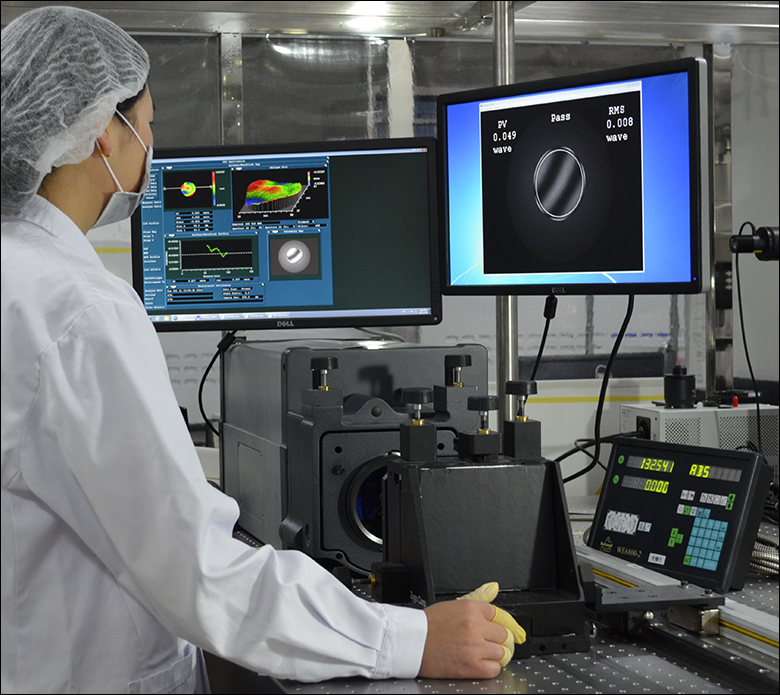
Figure 3.1 A Thorlabs technician measuring the irregularity of one of our singlets using a Zygo GPI-XP/D Interferometer.
Introduction
Thorlabs has a series of quality control procedures in order to ensure our singlets meet our standards and specifications. This starts with in-process inspections of the lens’ imaging capabilities and ends with a final inspection of surface quality and dimensions. Specifications for particular products can be found in their linked documentation by clicking the ![]() symbol. This tab will take you through the general process used to check for quality.
symbol. This tab will take you through the general process used to check for quality.
Singlet Quality Practices
In-process inspection begins once the singlet has been shaped to specifications. Focal length, surface irregularity, and surface power are checked, following sampling plan Level VI given in MIL-PRF-13830B (see below). These three specifications are imperative for proper imaging. Surface irregularity of parts is kept to below either a quarter wavelength or a half wavelength at 633 nm, depending on the material of the singlet. In Table 3.3 is a graph of over 200 batches of singlets with irregularity data of both their front and back sides.
At this point, some uncoated singlets will proceed to final inspection, while others will receive an antireflective (AR) coating. The application of optical coatings has its own in-process inspections. To ensure the AR coating is applied properly, we verify both reflectance and transmission performance by scanning witness pieces using spectrophotometry; the material of these 2 mm thick witness samples matches the other parts in the run. For reflectance verification, we use at least one witness sample for each coating run. Transmitting optics receive two AR coatings, one on each surface, so for the verification of transmission, we use one witness sample that is also coated on both of its sides. Large runs use multiple witness samples to ensure the uniformity across the deposition chamber. By testing coating performance during every run, variance over time is kept low. To see how coatings vary, see Table 3.2.
Final inspection of both uncoated and AR-coated singlets includes a batch check of diameter and thickness and a 100% visual check to ensure that the surface quality, chamfer, and clear aperture meet our published specifications. While surface quality is cosmetic to a degree, scratches, digs, and other inclusions in the surface of a part can increase the chances of damage to the singlet when used with high-power sources. These inspections are done in a clean, dark room under lighting that meets the requirements of MIL-PRF-13830B. Inspection under a single light source in a dark room allows for inconsistencies in the glass to be located without being obscured by glare or reflections.
MIL-PRF-13830B: Performance Specifications for Optical Components
MIL-PRF-13830B is a document created by the U.S. Army Armament Research, Development and Engineering Center's Defense Quality and Standardization Office for the specifications covering how finished optical components should be manufactured, assembled, and inspected. While primarily for use in letting the military dictate how products they use can be incorporated into their equipment, these standards have been adopted by many optics manufacturers. To download a copy of the full document,
| Table 3.2 Coating Variance | Table 3.3 Singlet Irregularity |
||||
| -A Coating 350 nm to 700 nm |
-B Coating 650 nm to 1050 nm |
-C Coating 1050 nm to 1700 nm |
|||
| Transmission |  Click to Enlarge |
 Click to Enlarge |
 Click to Enlarge |
 Click to Enlarge |
|
| Reflectance |  Click to Enlarge |
 Click to Enlarge |
 Click to Enlarge |
||
| Table 4.1 Damage Threshold Specifications | |
|---|---|
| Coating Designation (Item # Suffix) |
Damage Threshold |
| -A | 7.5 J/cm2 (532 nm, 10 ns, 10 Hz, Ø0.504 mm) |
Damage Threshold Data for Thorlabs' A-Coated N-BK7 Singlet Lenses
The specifications in Table 4.1 are measured data for Thorlabs' A-coated N-BK7 spherical singlet lenses. Damage threshold specifications are constant for all A-coated N-BK7 lenses, regardless of the size or focal length of the lens.
Laser Induced Damage Threshold Tutorial
The following is a general overview of how laser induced damage thresholds are measured and how the values may be utilized in determining the appropriateness of an optic for a given application. When choosing optics, it is important to understand the Laser Induced Damage Threshold (LIDT) of the optics being used. The LIDT for an optic greatly depends on the type of laser you are using. Continuous wave (CW) lasers typically cause damage from thermal effects (absorption either in the coating or in the substrate). Pulsed lasers, on the other hand, often strip electrons from the lattice structure of an optic before causing thermal damage. Note that the guideline presented here assumes room temperature operation and optics in new condition (i.e., within scratch-dig spec, surface free of contamination, etc.). Because dust or other particles on the surface of an optic can cause damage at lower thresholds, we recommend keeping surfaces clean and free of debris. For more information on cleaning optics, please see our Optics Cleaning tutorial.
Testing Method
Thorlabs' LIDT testing is done in compliance with ISO/DIS 11254 and ISO 21254 specifications.
First, a low-power/energy beam is directed to the optic under test. The optic is exposed in 10 locations to this laser beam for 30 seconds (CW) or for a number of pulses (pulse repetition frequency specified). After exposure, the optic is examined by a microscope (~100X magnification) for any visible damage. The number of locations that are damaged at a particular power/energy level is recorded. Next, the power/energy is either increased or decreased and the optic is exposed at 10 new locations. This process is repeated until damage is observed. The damage threshold is then assigned to be the highest power/energy that the optic can withstand without causing damage. A histogram such as that shown in Figure 37B represents the testing of one BB1-E02 mirror.
Figure 37A This photograph shows a protected aluminum-coated mirror after LIDT testing. In this particular test, it handled 0.43 J/cm2 (1064 nm, 10 ns pulse, 10 Hz, Ø1.000 mm) before damage.
Figure 37B Example Exposure Histogram used to Determine the LIDT of
| Table 37C Example Test Data | |||
|---|---|---|---|
| Fluence | # of Tested Locations | Locations with Damage | Locations Without Damage |
| 1.50 J/cm2 | 10 | 0 | 10 |
| 1.75 J/cm2 | 10 | 0 | 10 |
| 2.00 J/cm2 | 10 | 0 | 10 |
| 2.25 J/cm2 | 10 | 1 | 9 |
| 3.00 J/cm2 | 10 | 1 | 9 |
| 5.00 J/cm2 | 10 | 9 | 1 |
According to the test, the damage threshold of the mirror was 2.00 J/cm2 (532 nm, 10 ns pulse, 10 Hz, Ø0.803 mm). Please keep in mind that these tests are performed on clean optics, as dirt and contamination can significantly lower the damage threshold of a component. While the test results are only representative of one coating run, Thorlabs specifies damage threshold values that account for coating variances.
Continuous Wave and Long-Pulse Lasers
When an optic is damaged by a continuous wave (CW) laser, it is usually due to the melting of the surface as a result of absorbing the laser's energy or damage to the optical coating (antireflection) [1]. Pulsed lasers with pulse lengths longer than 1 µs can be treated as CW lasers for LIDT discussions.
When pulse lengths are between 1 ns and 1 µs, laser-induced damage can occur either because of absorption or a dielectric breakdown (therefore, a user must check both CW and pulsed LIDT). Absorption is either due to an intrinsic property of the optic or due to surface irregularities; thus LIDT values are only valid for optics meeting or exceeding the surface quality specifications given by a manufacturer. While many optics can handle high power CW lasers, cemented (e.g., achromatic doublets) or highly absorptive (e.g., ND filters) optics tend to have lower CW damage thresholds. These lower thresholds are due to absorption or scattering in the cement or metal coating.

Figure 37D LIDT in linear power density vs. pulse length and spot size. For long pulses to CW, linear power density becomes a constant with spot size. This graph was obtained from [1].
Figure 37E Intensity Distribution of Uniform and Gaussian Beam Profiles
Pulsed lasers with high pulse repetition frequencies (PRF) may behave similarly to CW beams. Unfortunately, this is highly dependent on factors such as absorption and thermal diffusivity, so there is no reliable method for determining when a high PRF laser will damage an optic due to thermal effects. For beams with a high PRF both the average and peak powers must be compared to the equivalent CW power. Additionally, for highly transparent materials, there is little to no drop in the LIDT with increasing PRF.
In order to use the specified CW damage threshold of an optic, it is necessary to know the following:
- Wavelength of your laser
- Beam diameter of your beam (1/e2)
- Approximate intensity profile of your beam (e.g., Gaussian)
- Linear power density of your beam (total power divided by 1/e2 beam diameter)
Thorlabs expresses LIDT for CW lasers as a linear power density measured in W/cm. In this regime, the LIDT given as a linear power density can be applied to any beam diameter; one does not need to compute an adjusted LIDT to adjust for changes in spot size, as demonstrated in Figure 37D. Average linear power density can be calculated using this equation.
This calculation assumes a uniform beam intensity profile. You must now consider hotspots in the beam or other non-uniform intensity profiles and roughly calculate a maximum power density. For reference, a Gaussian beam typically has a maximum power density that is twice that of the uniform beam (see Figure 37E).
Now compare the maximum power density to that which is specified as the LIDT for the optic. If the optic was tested at a wavelength other than your operating wavelength, the damage threshold must be scaled appropriately. A good rule of thumb is that the damage threshold has a linear relationship with wavelength such that as you move to shorter wavelengths, the damage threshold decreases (i.e., a LIDT of 10 W/cm at 1310 nm scales to 5 W/cm at 655 nm):
While this rule of thumb provides a general trend, it is not a quantitative analysis of LIDT vs wavelength. In CW applications, for instance, damage scales more strongly with absorption in the coating and substrate, which does not necessarily scale well with wavelength. While the above procedure provides a good rule of thumb for LIDT values, please contact Tech Support if your wavelength is different from the specified LIDT wavelength. If your power density is less than the adjusted LIDT of the optic, then the optic should work for your application.
Please note that we have a buffer built in between the specified damage thresholds online and the tests which we have done, which accommodates variation between batches. Upon request, we can provide individual test information and a testing certificate. The damage analysis will be carried out on a similar optic (customer's optic will not be damaged). Testing may result in additional costs or lead times. Contact Tech Support for more information.
Pulsed Lasers
As previously stated, pulsed lasers typically induce a different type of damage to the optic than CW lasers. Pulsed lasers often do not heat the optic enough to damage it; instead, pulsed lasers produce strong electric fields capable of inducing dielectric breakdown in the material. Unfortunately, it can be very difficult to compare the LIDT specification of an optic to your laser. There are multiple regimes in which a pulsed laser can damage an optic and this is based on the laser's pulse length. The highlighted columns in Table 37F outline the relevant pulse lengths for our specified LIDT values.
Pulses shorter than 10-9 s cannot be compared to our specified LIDT values with much reliability. In this ultra-short-pulse regime various mechanics, such as multiphoton-avalanche ionization, take over as the predominate damage mechanism [2]. In contrast, pulses between 10-7 s and 10-4 s may cause damage to an optic either because of dielectric breakdown or thermal effects. This means that both CW and pulsed damage thresholds must be compared to the laser beam to determine whether the optic is suitable for your application.
| Table 37F Laser Induced Damage Regimes | ||||
|---|---|---|---|---|
| Pulse Duration | t < 10-9 s | 10-9 < t < 10-7 s | 10-7 < t < 10-4 s | t > 10-4 s |
| Damage Mechanism | Avalanche Ionization | Dielectric Breakdown | Dielectric Breakdown or Thermal | Thermal |
| Relevant Damage Specification | No Comparison (See Above) | Pulsed | Pulsed and CW | CW |
When comparing an LIDT specified for a pulsed laser to your laser, it is essential to know the following:
Figure 37G LIDT in energy density vs. pulse length and spot size. For short pulses, energy density becomes a constant with spot size. This graph was obtained from [1].
- Wavelength of your laser
- Energy density of your beam (total energy divided by 1/e2 area)
- Pulse length of your laser
- Pulse repetition frequency (prf) of your laser
- Beam diameter of your laser (1/e2 )
- Approximate intensity profile of your beam (e.g., Gaussian)
The energy density of your beam should be calculated in terms of J/cm2. Figure 37G shows why expressing the LIDT as an energy density provides the best metric for short pulse sources. In this regime, the LIDT given as an energy density can be applied to any beam diameter; one does not need to compute an adjusted LIDT to adjust for changes in spot size. This calculation assumes a uniform beam intensity profile. You must now adjust this energy density to account for hotspots or other nonuniform intensity profiles and roughly calculate a maximum energy density. For reference a Gaussian beam typically has a maximum energy density that is twice that of the 1/e2 beam.
Now compare the maximum energy density to that which is specified as the LIDT for the optic. If the optic was tested at a wavelength other than your operating wavelength, the damage threshold must be scaled appropriately [3]. A good rule of thumb is that the damage threshold has an inverse square root relationship with wavelength such that as you move to shorter wavelengths, the damage threshold decreases (i.e., a LIDT of 1 J/cm2 at 1064 nm scales to 0.7 J/cm2 at 532 nm):
You now have a wavelength-adjusted energy density, which you will use in the following step.
Beam diameter is also important to know when comparing damage thresholds. While the LIDT, when expressed in units of J/cm², scales independently of spot size; large beam sizes are more likely to illuminate a larger number of defects which can lead to greater variances in the LIDT [4]. For data presented here, a <1 mm beam size was used to measure the LIDT. For beams sizes greater than 5 mm, the LIDT (J/cm2) will not scale independently of beam diameter due to the larger size beam exposing more defects.
The pulse length must now be compensated for. The longer the pulse duration, the more energy the optic can handle. For pulse widths between 1 - 100 ns, an approximation is as follows:
Use this formula to calculate the Adjusted LIDT for an optic based on your pulse length. If your maximum energy density is less than this adjusted LIDT maximum energy density, then the optic should be suitable for your application. Keep in mind that this calculation is only used for pulses between 10-9 s and 10-7 s. For pulses between 10-7 s and 10-4 s, the CW LIDT must also be checked before deeming the optic appropriate for your application.
Please note that we have a buffer built in between the specified damage thresholds online and the tests which we have done, which accommodates variation between batches. Upon request, we can provide individual test information and a testing certificate. Contact Tech Support for more information.
[1] R. M. Wood, Optics and Laser Tech. 29, 517 (1998).
[2] Roger M. Wood, Laser-Induced Damage of Optical Materials (Institute of Physics Publishing, Philadelphia, PA, 2003).
[3] C. W. Carr et al., Phys. Rev. Lett. 91, 127402 (2003).
[4] N. Bloembergen, Appl. Opt. 12, 661 (1973).

In order to illustrate the process of determining whether a given laser system will damage an optic, a number of example calculations of laser induced damage threshold are given below. For assistance with performing similar calculations, we provide a spreadsheet calculator that can be downloaded by clicking the LIDT Calculator button. To use the calculator, enter the specified LIDT value of the optic under consideration and the relevant parameters of your laser system in the green boxes. The spreadsheet will then calculate a linear power density for CW and pulsed systems, as well as an energy density value for pulsed systems. These values are used to calculate adjusted, scaled LIDT values for the optics based on accepted scaling laws. This calculator assumes a Gaussian beam profile, so a correction factor must be introduced for other beam shapes (uniform, etc.). The LIDT scaling laws are determined from empirical relationships; their accuracy is not guaranteed. Remember that absorption by optics or coatings can significantly reduce LIDT in some spectral regions. These LIDT values are not valid for ultrashort pulses less than one nanosecond in duration.
Figure 71A A Gaussian beam profile has about twice the maximum intensity of a uniform beam profile.
CW Laser Example
Suppose that a CW laser system at 1319 nm produces a 0.5 W Gaussian beam that has a 1/e2 diameter of 10 mm. A naive calculation of the average linear power density of this beam would yield a value of 0.5 W/cm, given by the total power divided by the beam diameter:
However, the maximum power density of a Gaussian beam is about twice the maximum power density of a uniform beam, as shown in Figure 71A. Therefore, a more accurate determination of the maximum linear power density of the system is 1 W/cm.
An AC127-030-C achromatic doublet lens has a specified CW LIDT of 350 W/cm, as tested at 1550 nm. CW damage threshold values typically scale directly with the wavelength of the laser source, so this yields an adjusted LIDT value:
The adjusted LIDT value of 350 W/cm x (1319 nm / 1550 nm) = 298 W/cm is significantly higher than the calculated maximum linear power density of the laser system, so it would be safe to use this doublet lens for this application.
Pulsed Nanosecond Laser Example: Scaling for Different Pulse Durations
Suppose that a pulsed Nd:YAG laser system is frequency tripled to produce a 10 Hz output, consisting of 2 ns output pulses at 355 nm, each with 1 J of energy, in a Gaussian beam with a 1.9 cm beam diameter (1/e2). The average energy density of each pulse is found by dividing the pulse energy by the beam area:
As described above, the maximum energy density of a Gaussian beam is about twice the average energy density. So, the maximum energy density of this beam is ~0.7 J/cm2.
The energy density of the beam can be compared to the LIDT values of 1 J/cm2 and 3.5 J/cm2 for a BB1-E01 broadband dielectric mirror and an NB1-K08 Nd:YAG laser line mirror, respectively. Both of these LIDT values, while measured at 355 nm, were determined with a 10 ns pulsed laser at 10 Hz. Therefore, an adjustment must be applied for the shorter pulse duration of the system under consideration. As described on the previous tab, LIDT values in the nanosecond pulse regime scale with the square root of the laser pulse duration:
This adjustment factor results in LIDT values of 0.45 J/cm2 for the BB1-E01 broadband mirror and 1.6 J/cm2 for the Nd:YAG laser line mirror, which are to be compared with the 0.7 J/cm2 maximum energy density of the beam. While the broadband mirror would likely be damaged by the laser, the more specialized laser line mirror is appropriate for use with this system.
Pulsed Nanosecond Laser Example: Scaling for Different Wavelengths
Suppose that a pulsed laser system emits 10 ns pulses at 2.5 Hz, each with 100 mJ of energy at 1064 nm in a 16 mm diameter beam (1/e2) that must be attenuated with a neutral density filter. For a Gaussian output, these specifications result in a maximum energy density of 0.1 J/cm2. The damage threshold of an NDUV10A Ø25 mm, OD 1.0, reflective neutral density filter is 0.05 J/cm2 for 10 ns pulses at 355 nm, while the damage threshold of the similar NE10A absorptive filter is 10 J/cm2 for 10 ns pulses at 532 nm. As described on the previous tab, the LIDT value of an optic scales with the square root of the wavelength in the nanosecond pulse regime:
This scaling gives adjusted LIDT values of 0.08 J/cm2 for the reflective filter and 14 J/cm2 for the absorptive filter. In this case, the absorptive filter is the best choice in order to avoid optical damage.
Pulsed Microsecond Laser Example
Consider a laser system that produces 1 µs pulses, each containing 150 µJ of energy at a repetition rate of 50 kHz, resulting in a relatively high duty cycle of 5%. This system falls somewhere between the regimes of CW and pulsed laser induced damage, and could potentially damage an optic by mechanisms associated with either regime. As a result, both CW and pulsed LIDT values must be compared to the properties of the laser system to ensure safe operation.
If this relatively long-pulse laser emits a Gaussian 12.7 mm diameter beam (1/e2) at 980 nm, then the resulting output has a linear power density of 5.9 W/cm and an energy density of 1.2 x 10⁻⁴ J/cm2 per pulse. This can be compared to the LIDT values for a WPQ10E-980 polymer zero-order quarter-wave plate, which are 5 W/cm for CW radiation at 810 nm and 5 J/cm2 for a 10 ns pulse at 810 nm. As before, the CW LIDT of the optic scales linearly with the laser wavelength, resulting in an adjusted CW value of 6 W/cm at 980 nm. On the other hand, the pulsed LIDT scales with the square root of the laser wavelength and the square root of the pulse duration, resulting in an adjusted value of 55 J/cm2 for a 1 µs pulse at 980 nm. The pulsed LIDT of the optic is significantly greater than the energy density of the laser pulse, so individual pulses will not damage the wave plate. However, the large average linear power density of the laser system may cause thermal damage to the optic, much like a high-power CW beam.
| Recommended Mounting Options for Thorlabs Lenses | ||
|---|---|---|
| Item # | Mounts for Ø2 mm to Ø10 mm Optics | |
| Imperial | Metric | |
| (Various) | Fixed Lens Mounts and Mini-Series Fixed Lens Mounts for Small Optics, Ø5 mm to Ø10 mm | |
| (Various) | Small Optic Adapters for Use with Standard Fixed Lens Mounts, Ø2 mm to Ø10 mm | |
| Item # | Mounts for Ø1/2" (Ø12.7 mm) Optics | |
| Imperial | Metric | |
| LMR05 | LMR05/M | Fixed Lens Mount for Ø1/2" Optics |
| MLH05 | MLH05/M | Mini-Series Fixed Lens Mount for Ø1/2" Optics |
| LM05XY | LM05XY/M | Translating Lens Mount for Ø1/2" Optics |
| SCP05 | 16 mm Cage System, XY Translation Mount for Ø1/2" Optics | |
| (Various) | Ø1/2" Lens Tubes, Optional SM05RRC Retaining Ring for High-Curvature Lenses (See Below) |
|
| Item # | Mounts for Ø1" (Ø25.4 mm) Optics | |
| Imperial | Metric | |
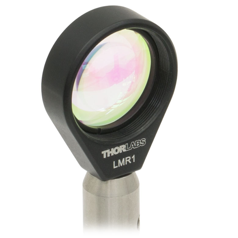
| LMR1 | LMR1/M | Fixed Lens Mount for Ø1" Optics |
| LM1XY | LM1XY/M | Translating Lens Mount for Ø1" Optics |
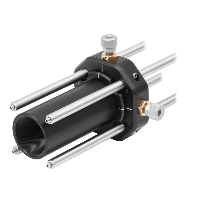
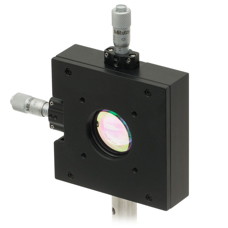
| ST1XY-S | ST1XY-S/M | Translating Lens Mount with Micrometer Drives (Other Drives Available) |
| CXY1A | 30 mm Cage System, XY Translation Mount for Ø1" Optics | |
| (Various) | Ø1" Lens Tubes, Optional SM1RRC Retaining Ring for High-Curvature Lenses (See Below) |
|
| Item # | Mount for Ø1.5" Optics | |
| Imperial | Metric | |
| LMR1.5 | LMR1.5/M | Fixed Lens Mount for Ø1.5" Optics |
| (Various) | Ø1.5" Lens Tubes, Optional SM1.5RR Retaining Ring for Ø1.5" Lens Tubes and Mounts |
|
| Item # | Mounts for Ø2" (Ø50.8 mm) Optics | |
| Imperial | Metric | |
| LMR2 | LMR2/M | Fixed Lens Mount for Ø2" Optics |
| LM2XY | LM2XY/M | Translating Lens Mount for Ø2" Optics |
| CXY2 | 60 mm Cage System, XY Translation Mount for Ø2" Optics |
|
| (Various) | Ø2" Lens Tubes, Optional SM2RRC Retaining Ring for High-Curvature Lenses (See Below) |
|
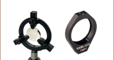
| Item # | Adjustable Optic Mounts | |
| Imperial | Metric | |
| LH1 | LH1/M | Adjustable Mount for Ø0.28" (Ø7.1 mm) to Ø1.80" (Ø45.7 mm) Optics |
| LH2 | LH2/M | Adjustable Mount for Ø0.77" (Ø19.6 mm) to Ø2.28" (Ø57.9 mm) Optics |
| VG100 | VG100/M | Adjustable Clamp for Ø0.5" (Ø13 mm) to Ø3.5" (Ø89 mm) Optics |
| SCL03 | SCL03/M | Self-Centering Mount for Ø0.15" (Ø3.8 mm) to Ø1.77" (Ø45.0 mm) Optics |
| SCL04 | SCL04/M | Self-Centering Mount for Ø0.15" (Ø3.8 mm) to Ø3.00" (Ø76.2 mm) Optics |
| LH160CA | LH160CA/M | Adjustable Mount for 60 mm Cage Systems, Ø0.50" (Ø13 mm) to Ø2.00" (Ø50.8 mm) Optics |
| SCL60CA | SCL60CA/M | Self-Centering Mount for 60 mm Cage Systems, Ø0.15" (Ø3.8 mm) to Ø1.77" (Ø45.0 mm) Optics |
Mounting High-Curvature Optics
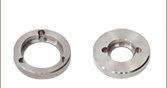
Thorlabs' retaining rings are used to secure unmounted optics within lens tubes or optic mounts. These rings are secured in position using a compatible spanner wrench. For flat or low-curvature optics, standard retaining rings manufactured from anodized aluminum are available from Ø5 mm to Ø4". For high-curvature optics, extra-thick retaining rings are available in Ø1/2", Ø1", and Ø2" sizes.
Extra-thick retaining rings offer several features that aid in mounting high-curvature optics such as aspheric lenses, short-focal-length plano-convex lenses, and condenser lenses. As shown in the animation to the right, the guide flange of the spanner wrench will collide with the surface of high-curvature lenses when using a standard retaining ring, potentially scratching the optic. This contact also creates a gap between the spanner wrench and retaining ring, preventing the ring from tightening correctly. Extra-thick retaining rings provide the necessary clearance for the spanner wrench to secure the lens without coming into contact with the optic surface.
| Posted Comments: | |
Paul Pulaski
(posted 2022-08-18 10:56:40.39) Hello, I purchased an LC1582 lens. Do you and can you provide a certificate of conformance for this lens? Our company is Wavefront Dynamics, ABQ, NM
Thanks,
Paul ksosnowski
(posted 2022-08-23 01:21:46.0) Thanks for reaching out to Thorlabs. The certificate is included on every Thorlabs Packing Slip, so you will receive a certification of conformance with the delivery of the order. If you are looking for a copy of certification for an order you already purchased, we will need the Thorlabs sales order number so we can produce the CoC. I have reached out directly to discuss this further. |
| Item # | Diameter | Focal Length | Dioptera | Radius of Curvature | Center Thickness | Edge Thicknessb | Back Focal Length | Reference Drawing |
|---|---|---|---|---|---|---|---|---|
| LC1054-A | 1/2" | -25.0 mm | -40.0 | -12.9 mm | 3.0 mm | 4.7 mm | -27.0 mm | 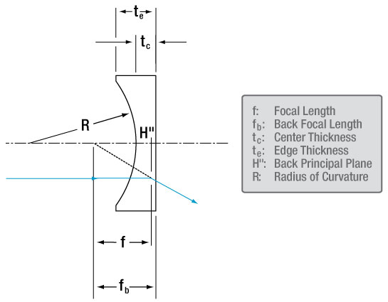 |
| LC1060-A | 1/2" | -30.0 mm | -33.3 | -15.4 mm | 3.0 mm | 4.4 mm | -32.0 mm | |
| LC1439-A | 1/2" | -50.0 mm | -20.0 | -25.7 mm | 3.5 mm | 4.3 mm | -52.3 mm |
| Item # | Diameter | Focal Length | Dioptera | Radius of Curvature | Center Thickness | Edge Thicknessb | Back Focal Length | Reference Drawing |
|---|---|---|---|---|---|---|---|---|
| LC1259-A | 25.0 mm | -50.0 mm | -20.0 | -25.7 mm | 3.5 mm | 6.7 mm | -52.3 mm | |
| LC1258-A | 25.0 mm | -75.0 mm | -13.3 | -38.6 mm | 3.5 mm | 5.6 mm | -77.3 mm | |
| LC1254-A | 25.0 mm | -100.0 mm | -10.0 | -51.5 mm | 4.0 mm | 5.5 mm | -102.6 mm |
| Item # | Diameter | Focal Length | Dioptera | Radius of Curvature | Center Thickness | Edge Thicknessb | Back Focal Length | Reference Drawing |
|---|---|---|---|---|---|---|---|---|
| LC1715-A | 1" | -50.0 mm | -20.0 | -25.7 mm | 3.5 mm | 6.9 mm | -52.3 mm | |
| LC1582-A | 1" | -75.0 mm | -13.3 | -38.6 mm | 3.5 mm | 5.6 mm | -77.3 mm | |
| LC1120-A | 1" | -100.0 mm | -10.0 | -51.5 mm | 4.0 mm | 5.6 mm | -102.6 mm |
| Item # | Diameter | Focal Length | Dioptera | Radius of Curvature | Center Thickness | Edge Thicknessb | Back Focal Length | Reference Drawing |
|---|---|---|---|---|---|---|---|---|
| LC1315-Ac | 2" | -75.0 mm | -13.3 | -38.6 mm | 3.5 mm | 13.0 mm | -77.3 mm | |
| LC1093-Ac | 2" | -100.0 mm | -10.0 | -51.5 mm | 4.0 mm | 10.7 mm | -102.6 mm | |
| LC1611-Ad | 2" | -150.0 mm | -6.7 | -77.2 mm | 4.0 mm | 8.3 mm | -152.6 mm |