 Products Home / Optical Elements / Optical Lenses / Cylindrical Lenses / Mounted Plano-Convex Round Cylindrical Lenses, N-BK7
Mounted Plano-Convex Round Cylindrical Lenses, N-BK7

- Used to Focus Light in One Dimension
- Ø1" Housing with a >21 mm Clear Aperture
- Available Uncoated or with One of Three AR Coatings
LJ1567RM-A
LJ1703RM-B
LJ1144RM-C
LJ1629RM


Please Wait
| Common Specifications | |
|---|---|
| Material | N-BK7a |
| Wavelength Range | Uncoated: 350 nm - 2.0 µm -A Coated: 350 - 700 nm -B Coated: 650 - 1050 nm -C Coated: 1050 - 1700 nm |
| Broadband AR Coating Reflectivityb | Ravg < 0.5% |
| Design Wavelength | 587.6 nm |
| Diameter | 25.4 mm (1") |
| Diameter Tolerance | +0.00/-0.10 mm |
| Clear Aperture | >21.0 mm |
| Focal Length Tolerance | ±1% |
| Surface Quality | 60-40 Scratch-Dig |
| Centration | ≤3 arcmin |
| Surface Flatness (Plano Side) | λ/2 |
| Surface Powerc (Convex Side) |
3λ/2 |
| Surface Irregularity (Convex Side) (Peak to Valley) |
λ |
| Damage Threshold | A: 7.5 J/cm2 (532 nm, 10 ns, 10 Hz, Ø0.456 mm) B: 7.5 J/cm2 (810 nm, 10 ns, 10 Hz, Ø0.144 mm) C: 7.5 J/cm2 (1542 nm, 10 ns, 10 Hz, Ø0.123 mm) |
 Zemax Files Zemax Files |
|---|
| Click on the red Document icon next to the item numbers below to access the Zemax file download. Our entire Zemax Catalog is also available. |
Features
- Round Geometry Enables Easy Mounting and Adjustment
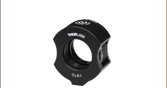
- Pre-Mounted in an Engraved, Black Anodized Aluminum Ring
- Full Contact Between Mounting Cell and Retaining Rings
- Optic Fabricated from N-BK7 Glass
- Focal Lengths from 50.0 mm to 1000.0 mm Available
- SM1 Lens Tube Compatible
- Enable Magnification in One Dimension
- Collimates & Circularizes the Output of a Laser Diode
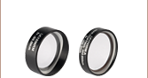
Like our N-BK7 plano-convex cylindrical lenses, these Ø1" positive round cylindrical lenses can be used to focus light but only in one dimension. However, they have the added advantage that they are epoxied into a round cell, allowing them to be mounted in our SM1 Lens Tubes or any Ø1" Lens Mounts.
The cell is black anodized and engraved with the part number, focal length, and coating information (if applicable). The wall thickness is designed to allow full contact with the cylindrical lens when using an SM1RR retaining ring to hold the lens.
One possible application is to use these lenses to focus fluorescence from a gas cell into a thin line imaged onto a photomultiplier tube. Alternatively, pairs of cylindrical lenses can be used to collimate and circularize the output of a laser diode. To minimize the introduction of spherical aberrations, collimated light should be incident on the curved surface when focusing it to a line, and a line source should be incident on the plano surface when collimating.
| Plano-Convex Cylindrical Lens Selection Guide | ||||
|---|---|---|---|---|
| Substrate | N-BK7 | UV Fused Silica | N-BK7 (Round) |
UV Fused Silica (Round) |
| AR Coating Range |
Uncoated 350 - 700 nm 650 - 1050 nm 1050 - 1700 nm |
Uncoated 245 - 400 nm 350 - 700 nm 650 - 1050 nm 1050 - 1700 nm |
Uncoated 350 - 700 nm 650 - 1050 nm 1050 - 1700 nm |
Uncoated 350 - 700 nm 650 - 1050 nm 1050 - 1700 nm |

| Item #a | Focal Lengthb |
Back Focal Length |
Radius | Center Thickness |
Housing Thickness |
Working Distanceb |
Reference Drawing |
|---|---|---|---|---|---|---|---|
| LJ1695RM | 50.0 mm | 45.5 mm | 25.8 mm | 6.8 mm | 8.3 mm | 44.2 mm | 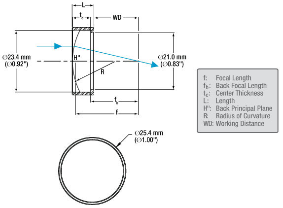 |
| LJ1703RM | 75.0 mm | 67.4 mm | 38.8 mm | 11.5 mm | 12.7 mm | 66.4 mm | |
| LJ1567RM | 100.0 mm | 96.6 mm | 51.7 mm | 5.2 mm | 8.2 mm | 95.2 mm | |
| LJ1629RM | 150.0 mm | 147.1 mm | 77.5 mm | 4.5 mm | 5.8 mm | 145.7 mm | |
| LJ1653RM | 200.0 mm | 197.3 mm | 103.4 mm | 4.1 mm | 5.8 mm | 196.0 mm | |
| LJ1267RM | 250.0 mm | 245.7 mm | 129.2 mm | 6.5 mm | 8.3 mm | 244.3 mm | |
| LJ1558RM | 300.0 mm | 297.7 mm | 155.1 mm | 3.8 mm | 5.8 mm | 296.3 mm | |
| LJ1363RM | 400.0 mm | 397.7 mm | 206.7 mm | 3.5 mm | 5.8 mm | 396.3 mm | |
| LJ1144RM | 500.0 mm | 497.7 mm | 258.4 mm | 3.4 mm | 5.8 mm | 496.4 mm | |
| LJ1516RM | 1000.0 mm | 997.9 mm | 516.8 mm | 3.2 mm | 5.8 mm | 996.5 mm |
| Common Specifications | |
|---|---|
| Material | N-BK7 |
| Wavelength Range | Uncoated: 350 nm - 2.0 µm -A Coating: 350 - 700 nm -B Coating: 650 - 1050 nm -C Coating: 1050 - 1700 nm |
| Broadband AR Coating Reflectivitya | Ravg < 0.5% |
| Design Wavelength | 587.6 nm |
| Diameter | 25.4 mm (1") |
| Diameter Tolerance | +0.00/-0.10 mm |
| Clear Aperture | >21.0 mm |
| Focal Length Tolerance | ±1% |
| Surface Quality | 60-40 Scratch-Dig |
| Centration | ≤3 arcmin |
| Surface Flatness (Plano Side) | λ/2 |
| Surface Power (Convex Side)b | 3λ/2 |
| Surface Irregularity (Convex Side) (Peak to Valley) |
λ |
All of our round cylindrical lenses can be ordered uncoated or with one of the following broadband AR coatings: -A: 350 - 700 nm, -B: 650 - 1050 nm, or -C: 1050 - 1700 nm.
These high performance multilayer AR coatings have an average reflectance of less than 0.5% (per surface) across the specified wavelength ranges and provide good performance for angles of incidence (AOI) between 0° and 30° (0.5 NA). The central peak in each curve is less than 0.25%. For optics intended to be used with larger incident angles, consider using a custom coating optimized for a 45° AOI; this custom coating is effective for use with angles of incidence between 25° and 52°. The Broadband AR Coatings plot indicates the performance of the standard coatings in this family as a function of wavelength. Broadband coatings have a typical absorption of 0.25%, which is not shown in the reflectivity plots.

Click to Enlarge
Click Here for Raw Data
The blue shaded region indicates the specified 650 - 1050 nm wavelength range for optimum performance.
Click to Enlarge
Click Here for Raw Data
The blue shaded region indicates the specified 350 - 700 nm wavelength range for optimum performance.
Click to Enlarge
Click Here for Raw Data
The blue shaded region indicates the specified 1050 - 1700 nm wavelength range for optimum performance.
| Table 4.1 Damage Threshold Specifications | |
|---|---|
| Coating Designation (Item # Suffix) |
Damage Threshold |
| -A | 7.5 J/cm2 (532 nm, 10 ns, 10 Hz, Ø0.456 mm) |
| -B | 7.5 J/cm2 (810 nm, 10 ns, 10 Hz, Ø0.144 mm) |
| -C | 7.5 J/cm2 (1542 nm, 10 ns, 10 Hz, Ø0.123 mm) |
Damage Threshold Data for Thorlabs' N-BK7 Lenses
The specifications in Table 4.1 are measured data for Thorlabs' N-BK7 lenses. Damage threshold specifications are constant for all N-BK7 lenses, regardless of the size or the focal length of the lens.
Laser Induced Damage Threshold Tutorial
The following is a general overview of how laser induced damage thresholds are measured and how the values may be utilized in determining the appropriateness of an optic for a given application. When choosing optics, it is important to understand the Laser Induced Damage Threshold (LIDT) of the optics being used. The LIDT for an optic greatly depends on the type of laser you are using. Continuous wave (CW) lasers typically cause damage from thermal effects (absorption either in the coating or in the substrate). Pulsed lasers, on the other hand, often strip electrons from the lattice structure of an optic before causing thermal damage. Note that the guideline presented here assumes room temperature operation and optics in new condition (i.e., within scratch-dig spec, surface free of contamination, etc.). Because dust or other particles on the surface of an optic can cause damage at lower thresholds, we recommend keeping surfaces clean and free of debris. For more information on cleaning optics, please see our Optics Cleaning tutorial.
Testing Method
Thorlabs' LIDT testing is done in compliance with ISO/DIS 11254 and ISO 21254 specifications.
First, a low-power/energy beam is directed to the optic under test. The optic is exposed in 10 locations to this laser beam for 30 seconds (CW) or for a number of pulses (pulse repetition frequency specified). After exposure, the optic is examined by a microscope (~100X magnification) for any visible damage. The number of locations that are damaged at a particular power/energy level is recorded. Next, the power/energy is either increased or decreased and the optic is exposed at 10 new locations. This process is repeated until damage is observed. The damage threshold is then assigned to be the highest power/energy that the optic can withstand without causing damage. A histogram such as that shown in Figure 37B represents the testing of one BB1-E02 mirror.
Figure 37A This photograph shows a protected aluminum-coated mirror after LIDT testing. In this particular test, it handled 0.43 J/cm2 (1064 nm, 10 ns pulse, 10 Hz, Ø1.000 mm) before damage.
Figure 37B Example Exposure Histogram used to Determine the LIDT of
| Table 37C Example Test Data | |||
|---|---|---|---|
| Fluence | # of Tested Locations | Locations with Damage | Locations Without Damage |
| 1.50 J/cm2 | 10 | 0 | 10 |
| 1.75 J/cm2 | 10 | 0 | 10 |
| 2.00 J/cm2 | 10 | 0 | 10 |
| 2.25 J/cm2 | 10 | 1 | 9 |
| 3.00 J/cm2 | 10 | 1 | 9 |
| 5.00 J/cm2 | 10 | 9 | 1 |
According to the test, the damage threshold of the mirror was 2.00 J/cm2 (532 nm, 10 ns pulse, 10 Hz, Ø0.803 mm). Please keep in mind that these tests are performed on clean optics, as dirt and contamination can significantly lower the damage threshold of a component. While the test results are only representative of one coating run, Thorlabs specifies damage threshold values that account for coating variances.
Continuous Wave and Long-Pulse Lasers
When an optic is damaged by a continuous wave (CW) laser, it is usually due to the melting of the surface as a result of absorbing the laser's energy or damage to the optical coating (antireflection) [1]. Pulsed lasers with pulse lengths longer than 1 µs can be treated as CW lasers for LIDT discussions.
When pulse lengths are between 1 ns and 1 µs, laser-induced damage can occur either because of absorption or a dielectric breakdown (therefore, a user must check both CW and pulsed LIDT). Absorption is either due to an intrinsic property of the optic or due to surface irregularities; thus LIDT values are only valid for optics meeting or exceeding the surface quality specifications given by a manufacturer. While many optics can handle high power CW lasers, cemented (e.g., achromatic doublets) or highly absorptive (e.g., ND filters) optics tend to have lower CW damage thresholds. These lower thresholds are due to absorption or scattering in the cement or metal coating.

Figure 37D LIDT in linear power density vs. pulse length and spot size. For long pulses to CW, linear power density becomes a constant with spot size. This graph was obtained from [1].
Figure 37E Intensity Distribution of Uniform and Gaussian Beam Profiles
Pulsed lasers with high pulse repetition frequencies (PRF) may behave similarly to CW beams. Unfortunately, this is highly dependent on factors such as absorption and thermal diffusivity, so there is no reliable method for determining when a high PRF laser will damage an optic due to thermal effects. For beams with a high PRF both the average and peak powers must be compared to the equivalent CW power. Additionally, for highly transparent materials, there is little to no drop in the LIDT with increasing PRF.
In order to use the specified CW damage threshold of an optic, it is necessary to know the following:
- Wavelength of your laser
- Beam diameter of your beam (1/e2)
- Approximate intensity profile of your beam (e.g., Gaussian)
- Linear power density of your beam (total power divided by 1/e2 beam diameter)
Thorlabs expresses LIDT for CW lasers as a linear power density measured in W/cm. In this regime, the LIDT given as a linear power density can be applied to any beam diameter; one does not need to compute an adjusted LIDT to adjust for changes in spot size, as demonstrated in Figure 37D. Average linear power density can be calculated using this equation.
This calculation assumes a uniform beam intensity profile. You must now consider hotspots in the beam or other non-uniform intensity profiles and roughly calculate a maximum power density. For reference, a Gaussian beam typically has a maximum power density that is twice that of the uniform beam (see Figure 37E).
Now compare the maximum power density to that which is specified as the LIDT for the optic. If the optic was tested at a wavelength other than your operating wavelength, the damage threshold must be scaled appropriately. A good rule of thumb is that the damage threshold has a linear relationship with wavelength such that as you move to shorter wavelengths, the damage threshold decreases (i.e., a LIDT of 10 W/cm at 1310 nm scales to 5 W/cm at 655 nm):
While this rule of thumb provides a general trend, it is not a quantitative analysis of LIDT vs wavelength. In CW applications, for instance, damage scales more strongly with absorption in the coating and substrate, which does not necessarily scale well with wavelength. While the above procedure provides a good rule of thumb for LIDT values, please contact Tech Support if your wavelength is different from the specified LIDT wavelength. If your power density is less than the adjusted LIDT of the optic, then the optic should work for your application.
Please note that we have a buffer built in between the specified damage thresholds online and the tests which we have done, which accommodates variation between batches. Upon request, we can provide individual test information and a testing certificate. The damage analysis will be carried out on a similar optic (customer's optic will not be damaged). Testing may result in additional costs or lead times. Contact Tech Support for more information.
Pulsed Lasers
As previously stated, pulsed lasers typically induce a different type of damage to the optic than CW lasers. Pulsed lasers often do not heat the optic enough to damage it; instead, pulsed lasers produce strong electric fields capable of inducing dielectric breakdown in the material. Unfortunately, it can be very difficult to compare the LIDT specification of an optic to your laser. There are multiple regimes in which a pulsed laser can damage an optic and this is based on the laser's pulse length. The highlighted columns in Table 37F outline the relevant pulse lengths for our specified LIDT values.
Pulses shorter than 10-9 s cannot be compared to our specified LIDT values with much reliability. In this ultra-short-pulse regime various mechanics, such as multiphoton-avalanche ionization, take over as the predominate damage mechanism [2]. In contrast, pulses between 10-7 s and 10-4 s may cause damage to an optic either because of dielectric breakdown or thermal effects. This means that both CW and pulsed damage thresholds must be compared to the laser beam to determine whether the optic is suitable for your application.
| Table 37F Laser Induced Damage Regimes | ||||
|---|---|---|---|---|
| Pulse Duration | t < 10-9 s | 10-9 < t < 10-7 s | 10-7 < t < 10-4 s | t > 10-4 s |
| Damage Mechanism | Avalanche Ionization | Dielectric Breakdown | Dielectric Breakdown or Thermal | Thermal |
| Relevant Damage Specification | No Comparison (See Above) | Pulsed | Pulsed and CW | CW |
When comparing an LIDT specified for a pulsed laser to your laser, it is essential to know the following:
Figure 37G LIDT in energy density vs. pulse length and spot size. For short pulses, energy density becomes a constant with spot size. This graph was obtained from [1].
- Wavelength of your laser
- Energy density of your beam (total energy divided by 1/e2 area)
- Pulse length of your laser
- Pulse repetition frequency (prf) of your laser
- Beam diameter of your laser (1/e2 )
- Approximate intensity profile of your beam (e.g., Gaussian)
The energy density of your beam should be calculated in terms of J/cm2. Figure 37G shows why expressing the LIDT as an energy density provides the best metric for short pulse sources. In this regime, the LIDT given as an energy density can be applied to any beam diameter; one does not need to compute an adjusted LIDT to adjust for changes in spot size. This calculation assumes a uniform beam intensity profile. You must now adjust this energy density to account for hotspots or other nonuniform intensity profiles and roughly calculate a maximum energy density. For reference a Gaussian beam typically has a maximum energy density that is twice that of the 1/e2 beam.
Now compare the maximum energy density to that which is specified as the LIDT for the optic. If the optic was tested at a wavelength other than your operating wavelength, the damage threshold must be scaled appropriately [3]. A good rule of thumb is that the damage threshold has an inverse square root relationship with wavelength such that as you move to shorter wavelengths, the damage threshold decreases (i.e., a LIDT of 1 J/cm2 at 1064 nm scales to 0.7 J/cm2 at 532 nm):
You now have a wavelength-adjusted energy density, which you will use in the following step.
Beam diameter is also important to know when comparing damage thresholds. While the LIDT, when expressed in units of J/cm², scales independently of spot size; large beam sizes are more likely to illuminate a larger number of defects which can lead to greater variances in the LIDT [4]. For data presented here, a <1 mm beam size was used to measure the LIDT. For beams sizes greater than 5 mm, the LIDT (J/cm2) will not scale independently of beam diameter due to the larger size beam exposing more defects.
The pulse length must now be compensated for. The longer the pulse duration, the more energy the optic can handle. For pulse widths between 1 - 100 ns, an approximation is as follows:
Use this formula to calculate the Adjusted LIDT for an optic based on your pulse length. If your maximum energy density is less than this adjusted LIDT maximum energy density, then the optic should be suitable for your application. Keep in mind that this calculation is only used for pulses between 10-9 s and 10-7 s. For pulses between 10-7 s and 10-4 s, the CW LIDT must also be checked before deeming the optic appropriate for your application.
Please note that we have a buffer built in between the specified damage thresholds online and the tests which we have done, which accommodates variation between batches. Upon request, we can provide individual test information and a testing certificate. Contact Tech Support for more information.
[1] R. M. Wood, Optics and Laser Tech. 29, 517 (1998).
[2] Roger M. Wood, Laser-Induced Damage of Optical Materials (Institute of Physics Publishing, Philadelphia, PA, 2003).
[3] C. W. Carr et al., Phys. Rev. Lett. 91, 127402 (2003).
[4] N. Bloembergen, Appl. Opt. 12, 661 (1973).

In order to illustrate the process of determining whether a given laser system will damage an optic, a number of example calculations of laser induced damage threshold are given below. For assistance with performing similar calculations, we provide a spreadsheet calculator that can be downloaded by clicking the LIDT Calculator button. To use the calculator, enter the specified LIDT value of the optic under consideration and the relevant parameters of your laser system in the green boxes. The spreadsheet will then calculate a linear power density for CW and pulsed systems, as well as an energy density value for pulsed systems. These values are used to calculate adjusted, scaled LIDT values for the optics based on accepted scaling laws. This calculator assumes a Gaussian beam profile, so a correction factor must be introduced for other beam shapes (uniform, etc.). The LIDT scaling laws are determined from empirical relationships; their accuracy is not guaranteed. Remember that absorption by optics or coatings can significantly reduce LIDT in some spectral regions. These LIDT values are not valid for ultrashort pulses less than one nanosecond in duration.
Figure 71A A Gaussian beam profile has about twice the maximum intensity of a uniform beam profile.
CW Laser Example
Suppose that a CW laser system at 1319 nm produces a 0.5 W Gaussian beam that has a 1/e2 diameter of 10 mm. A naive calculation of the average linear power density of this beam would yield a value of 0.5 W/cm, given by the total power divided by the beam diameter:
However, the maximum power density of a Gaussian beam is about twice the maximum power density of a uniform beam, as shown in Figure 71A. Therefore, a more accurate determination of the maximum linear power density of the system is 1 W/cm.
An AC127-030-C achromatic doublet lens has a specified CW LIDT of 350 W/cm, as tested at 1550 nm. CW damage threshold values typically scale directly with the wavelength of the laser source, so this yields an adjusted LIDT value:
The adjusted LIDT value of 350 W/cm x (1319 nm / 1550 nm) = 298 W/cm is significantly higher than the calculated maximum linear power density of the laser system, so it would be safe to use this doublet lens for this application.
Pulsed Nanosecond Laser Example: Scaling for Different Pulse Durations
Suppose that a pulsed Nd:YAG laser system is frequency tripled to produce a 10 Hz output, consisting of 2 ns output pulses at 355 nm, each with 1 J of energy, in a Gaussian beam with a 1.9 cm beam diameter (1/e2). The average energy density of each pulse is found by dividing the pulse energy by the beam area:
As described above, the maximum energy density of a Gaussian beam is about twice the average energy density. So, the maximum energy density of this beam is ~0.7 J/cm2.
The energy density of the beam can be compared to the LIDT values of 1 J/cm2 and 3.5 J/cm2 for a BB1-E01 broadband dielectric mirror and an NB1-K08 Nd:YAG laser line mirror, respectively. Both of these LIDT values, while measured at 355 nm, were determined with a 10 ns pulsed laser at 10 Hz. Therefore, an adjustment must be applied for the shorter pulse duration of the system under consideration. As described on the previous tab, LIDT values in the nanosecond pulse regime scale with the square root of the laser pulse duration:
This adjustment factor results in LIDT values of 0.45 J/cm2 for the BB1-E01 broadband mirror and 1.6 J/cm2 for the Nd:YAG laser line mirror, which are to be compared with the 0.7 J/cm2 maximum energy density of the beam. While the broadband mirror would likely be damaged by the laser, the more specialized laser line mirror is appropriate for use with this system.
Pulsed Nanosecond Laser Example: Scaling for Different Wavelengths
Suppose that a pulsed laser system emits 10 ns pulses at 2.5 Hz, each with 100 mJ of energy at 1064 nm in a 16 mm diameter beam (1/e2) that must be attenuated with a neutral density filter. For a Gaussian output, these specifications result in a maximum energy density of 0.1 J/cm2. The damage threshold of an NDUV10A Ø25 mm, OD 1.0, reflective neutral density filter is 0.05 J/cm2 for 10 ns pulses at 355 nm, while the damage threshold of the similar NE10A absorptive filter is 10 J/cm2 for 10 ns pulses at 532 nm. As described on the previous tab, the LIDT value of an optic scales with the square root of the wavelength in the nanosecond pulse regime:
This scaling gives adjusted LIDT values of 0.08 J/cm2 for the reflective filter and 14 J/cm2 for the absorptive filter. In this case, the absorptive filter is the best choice in order to avoid optical damage.
Pulsed Microsecond Laser Example
Consider a laser system that produces 1 µs pulses, each containing 150 µJ of energy at a repetition rate of 50 kHz, resulting in a relatively high duty cycle of 5%. This system falls somewhere between the regimes of CW and pulsed laser induced damage, and could potentially damage an optic by mechanisms associated with either regime. As a result, both CW and pulsed LIDT values must be compared to the properties of the laser system to ensure safe operation.
If this relatively long-pulse laser emits a Gaussian 12.7 mm diameter beam (1/e2) at 980 nm, then the resulting output has a linear power density of 5.9 W/cm and an energy density of 1.2 x 10⁻⁴ J/cm2 per pulse. This can be compared to the LIDT values for a WPQ10E-980 polymer zero-order quarter-wave plate, which are 5 W/cm for CW radiation at 810 nm and 5 J/cm2 for a 10 ns pulse at 810 nm. As before, the CW LIDT of the optic scales linearly with the laser wavelength, resulting in an adjusted CW value of 6 W/cm at 980 nm. On the other hand, the pulsed LIDT scales with the square root of the laser wavelength and the square root of the pulse duration, resulting in an adjusted value of 55 J/cm2 for a 1 µs pulse at 980 nm. The pulsed LIDT of the optic is significantly greater than the energy density of the laser pulse, so individual pulses will not damage the wave plate. However, the large average linear power density of the laser system may cause thermal damage to the optic, much like a high-power CW beam.
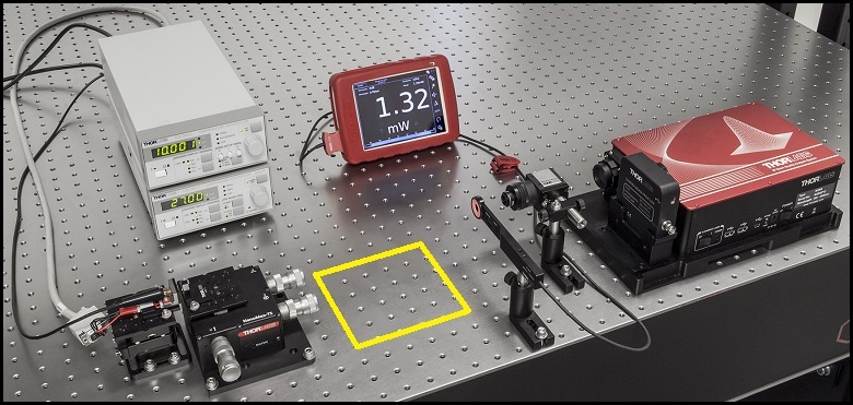
Click to Enlarge
Figure 168A The beam circularization systems were placed in the area of the experimental setup highlighted by the yellow rectangle.

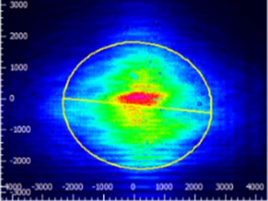
Comparison of Circularization Techniques for Elliptical Beams
Edge-emitting laser diodes emit elliptical beams as a consequence of the rectangular cross sections of their emission apertures. The component of the beam corresponding to the narrower dimension of the aperture has a greater divergence angle than the orthogonal beam component. As one component diverges more rapidly than the other, the beam shape is elliptical rather than circular.
Elliptical beam shapes can be undesirable, as the spot size of the focused beam is larger than if the beam were circular, and as larger spot sizes have lower irradiances (power per area). Techniques for circularizing an elliptical beam include those based on a pair of cylindrical lenses, an anamorphic prism pair, or a spatial filter. This work investigated all three approaches. The characteristics of the circularized beams were evaluated by performing M2 measurements, wavefront measurements, and measuring the transmitted power.
While it was demonstrated that each circularization technique improves the circularity of the elliptical input beam, each technique was shown to provide a different balance of circularization, beam quality, and transmitted power. The results of this work, which are documented in this Lab Fact, indicate that an application's specific requirements will determine which is the best circularization technique to choose.
Experimental Design and Setup
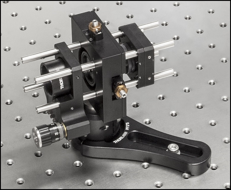
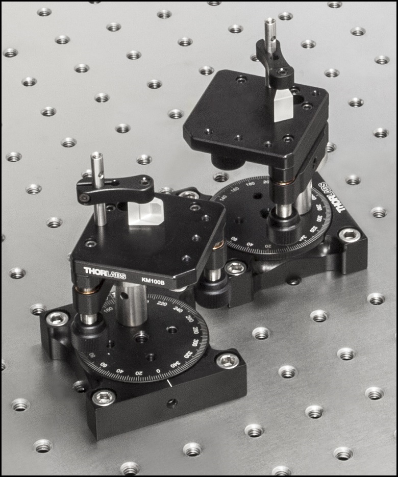
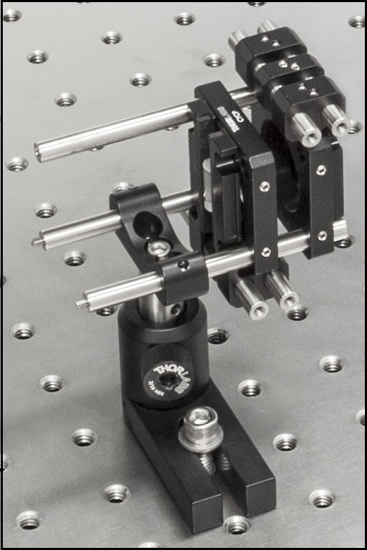
The experimental setup is shown in Figure 168A. The elliptically-shaped, collimated beam of a temperature-stabilized 670 nm laser diode was input to each of our circularization systems shown in Figures 168B through 168D. Collimation results in a low-divergence beam, but it does not affect the beam shape. Each system was based on one of the following:
- LJ1874L2-A and LJ1638L1-A Plano-Convex Convex Cylindrical Lenses (Figure 168B)
- PS873-A Unmounted Anamorphic Prism Pair (Figure 168C)
- Previous Generation KT310 Spatial Filter System with P5S Ø5 µm Pinhole (Figure 168D)
The beam circularization systems, shown in Figures 168B through 168D, were placed, one at a time, in the vacant spot in the setup highlighted by the yellow rectangle. With this arrangement, it was possible to use the same experimental conditions when evaluating each circularization technique, which allowed the performance of each to be directly compared with the others. This experimental constraint required the use of fixturing that was not optimally compact, as well as the use of an unmounted anamorphic prism pair, instead of a more convenient mounted and pre-aligned anamorphic prism pair.
The characteristics of the beams output by the different circularization systems were evaluated by making measurements using a power meter, a wavefront sensor, and an M2 system. In the image of the experimental setup shown in Figure 168A, all of these systems are shown on the right side of the optical table for illustrative purposes; they were used one at a time. The power meter was used to determine how much the beam circularization system attenuated the intensity of the input laser beam. The wavefront sensor provided a way to measure the aberrations of the output beam. The M2 system measurement describes the resemblance of the output beam to a Gaussian beam. Ideally, the circularization systems would not attenuate or aberrate the laser beam, and they would output a perfectly Gaussian beam.
Edge-emitting laser diodes also emit astigmatic beams, and it can be desirable to force the displaced focal points of the orthogonal beam components to overlap. Of the three circularization techniques investigated in this work, only the cylindrical lens pair can also compensate for astigmatism. The displacement between the focal spots of the orthogonal beam components were measured for each circularization technique. In the case of the cylindrical lens pair, their configuration was tuned to minimize the astigmatism in the laser beam. The astigmatism was reported as a normalized quantity.
Experimental Results
The experimental results are summarized in Table 168E, in which the green cells identify the best result in each category. Each circularization approach has its benefits. The best circularization technique for an application is determined by the system’s requirements for beam quality, transmitted optical power, and setup constraints.
Spatial filtering significantly improved the circularity and quality of the beam, but the beam had low transmitted power. The cylindrical lens pair provided a well-circularized beam and balanced circularization and beam quality with transmitted power. In addition, the cylindrical lens pair compensated for much of the beam's astigmatism. The circularity of the beam provided by the anamorphic prism pair compared well to that of the cylindrical lens pair. The beam output from the prisms had better M2 values and less wavefront error than the cylindrical lenses, but the transmitted power was lower.
| Table 168E Experimental Results | ||||||
|---|---|---|---|---|---|---|
| Method | Beam Intensity Profile | Circularitya | M2 Values | RMS Wavefront | Transmitted Power | Normalized Astigmatismb |
| Collimated Source Output (No Circularization Technique) |
 Click to Enlarge Scale in Microns |
0.36 | Y Axis: 1.63 |
0.17 | Not Applicable | 0.67 |
| Cylindrical Lens Pair | 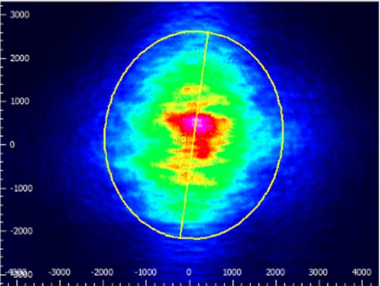 Click to Enlarge Scale in Microns |
0.84 | X Axis: 1.90 Y Axis: 1.93 |
0.30 | 91% | 0.06 |
| Anamorphic Prism Pair |
 Click to Enlarge Scale in Microns |
0.82 | X Axis: 1.60 Y Axis: 1.46 |
0.16 | 80% | 1.25 |
| Spatial Filter | 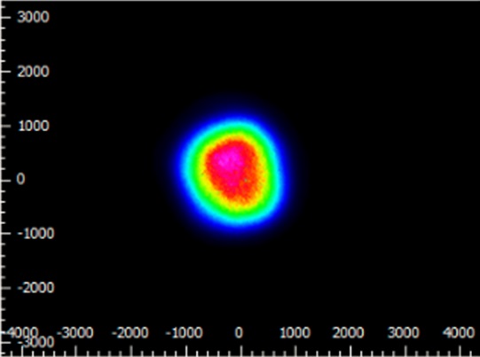 Click to Enlarge Scale in Microns |
0.93 | X Axis: 1.05 Y Axis: 1.10 |
0.10 | 34% | 0.36 |
Components used in each circularization system were chosen to allow the same experimental setup be used for all experiments. This had the desired effect of allowing the results of all circularization techniques to be directly compared; however, optimizing the setup for a circularization technique could have improved its performance. The mounts used for the collimating lens and the anamorphic prism pair enabled easy manipulation and integration into this experimental system. It is possible that using smaller mounts would improve results by allowing the members of each pair to be more precisely positioned with respect to one another. In addition, using made-to-order cylindrical lenses with customized focal lengths may have improved the results of the cylindrical lens pair circularization system. All results may have been affected by the use of the beam profiler software algorithm to determine the beam radii used in the circularity calculation.
Additional Information
Some information describing selection and configuration procedures for several components used in this experimental work can be accessed by clicking the following hyperlinks:
| Posted Comments: | |
Guillermo Garre Werner
(posted 2020-07-07 04:04:32.153) Hello,
I would like to know if there are Mounted Plano-Convex Round Cylindrical Lenses, N-BK7 with a focal length smaller than 50 mm.
Thank you. YLohia
(posted 2020-07-08 08:47:32.0) Hello, thank you for contacting Thorlabs. Custom optics can be requested by contacting your local Thorlabs Tech Support group (in your case europe@thorlabs.com). We will reach out to you directly to discuss the possibility of offering this. ad.agbur
(posted 2018-03-27 14:21:01.71) Hi. I concur with micke.malmstrom. Some kinf of marking indicating the "principal plane" either in the mount or side of the lens for unmounted indicating would be extremely useful. Also and equally important: how good are these lenses centered in the mount (or with respect to its own circular perimeter). Is it possible thar the lens' principal axis is shifted from the mount's (or its own diameter)?
https://www.dropbox.com/s/gjvgi705dnxltnc/Ejemplo_lente_Cil%C3%ADndrica_Desalineada.png?dl=0 nbayconich
(posted 2018-04-04 04:59:00.0) Thank you for contacting Thorlabs. We do not have a tolerance at the moment for the position of the optical axis relative to the mechanical axis of our mounted cylindrical lenses. Thank you for your suggestion in regards to marking the optical axis of the lens on the side of mount. I will reach out to you directly regarding our custom capabilities. micke.malmstrom
(posted 2016-04-28 10:35:10.923) It would be really nice if you could make some markings on both the lens-holders and the lenses so that one can align the it easier in the 0 and 90 deg position. Like you have for the waveplates eg AHWP10M-980
Thanks/M besembeson
(posted 2016-04-28 09:21:06.0) Response from Bweh at Thorlabs USA: This will actually add convenience in the integration into setups. We will review your suggestion. The CLR1 should help in proper alignment: http://www.thorlabs.com/newgrouppage9.cfm?objectgroup_ID=4113 robert.roy
(posted 2015-12-10 19:36:50.3) Hi there I am just wondering how easy is it for the plano convex lens to be held in the 1" lens holder and make sure that the lens remains upright? jlow
(posted 2015-12-10 04:10:26.0) Response from Jeremy at Thorlabs: With the SM1 threaded mounts, you are going to need some trial and error to ensure the lens final position is right. You can also use mounts such as the FMP1 that uses a setscrew to hold the optic. It's going to be a lot easier to keep the lens position with such a mount. bdada
(posted 2011-10-06 20:29:00.0) Response from Buki at Thorlabs:
Thank you for your feedback. We do not have any plano convex lenses with a 10m focal lens. We will contact you to learn more about your application so we can determine how to assist you. antony.lee
(posted 2011-10-06 10:11:48.0) Do you manufacture plano-convex cylindrical lenses with 10m focal length (and 1in diameter)? Thanks per advance. jens
(posted 2009-05-25 09:42:35.0) A response from Jens at Thorlabs: Yes, it has been added to the web page. You can find it using the search function and typing in the part number or by following this link, http://www.thorlabs.com/NewGroupPage9.cfm?ObjectGroup_ID=246&pn=CLR1&CFID=35450789&CFTOKEN=55397831 user
(posted 2009-05-25 08:53:27.0) Are there any news about the new mount CRL1 for the cylindrical lenses? jens
(posted 2009-05-13 16:06:37.0) A response from Jens at Thorlabs: Sorry for the delay, I can send you a prototype of our new mount CRL1 which we designed for these items. The product should appear on our web page in not more than a week. user
(posted 2009-05-08 22:27:21.0) Great idea with the lens but I have the same issue. The optics guy is a genius but no one told the mechanical guy to make a holder :-) When will the holder be in your catalog? jens
(posted 2009-05-07 19:08:51.0) An answer from Jens at Thorlabs: you are completely right that this product needs to be added as soon as possible. During the release process for these lenses the mounting options were checked as well but the design has unfortunately not been completely finished yet. I can look for a prototype to get you a solution as soon as possible. If you are interested please contact me via techsupport@thorlabs.com. user
(posted 2009-05-07 18:58:24.0) Uhh guys.. how am I suppose to hold this lens. The existing cylindrical mount wont work and the rotation mounts/lens tubes you show in the related produts, which use retaining rings, dont hold very well on this curved surface. I need xy and rotation. Please tell your holder engineer to make a holder for this lens. |