 Products Home / Optical Elements / Optical Lenses / Aspheric Lenses: Molded & Precision Polished / Precision Polished Aspheric Lenses / High-NA Aspheres: CNC Polished, UV Fused Silica Substrate
High-NA Aspheres: CNC Polished, UV Fused Silica Substrate

- High Numerical Aperture of 0.65
- UV Fused Silica Substrate
- Uncoated or AR-Coated for 245 - 420 nm
- CNC Precision Polished
CNC Satisloh Grinder Shaping an Aspheric Lens
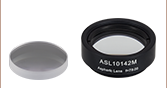
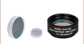
ASL1210
Ø12.5 mm Uncoated
ASL2520-UV
Ø25.0 mm UV Coating
ASL5040
Ø50.0 mm Uncoated


Please Wait
| Common Specificationsa | |
|---|---|
| Design Wavelength | 405 nm |
| Numerical Aperture (NA)b | 0.65 |
| Diameter Tolerance | +0.00/-0.05 mm |
| Focal Length Tolerance | ±1.0% |
| Surface Irregularity of Convex Surface |
<0.75 µm (RMS) |
| Surface Flatness of Plano Surface |
<λ/4 at 633 nm |
| Centration | <3 arcmin |
| Surface Quality | 60-40 Scratch-Dig |
| Index of Refraction (n)c | 1.4585 |
| Abbe Number (VD) | 67.82 ± 1.0% |
| f/#c,d | 0.87 |
| Substrate Material | UV Fused Silicae |
- Complete product-specific specifications are available by clicking on the blue Info Icons (
 ) below.
 - NA defined as the sine of the angle of the marginal ray.
- n and f/# are specified at the design wavelength.
- Obtained by dividing the focal length of the lens by its collimation clear aperture.
- Click link for detailed specifications on the substrate.
| Precision Aspheric Lenses Selection Guide | ||
|---|---|---|
| Substrate Material | NA | Mount |
| UV Fused Silica | 0.142 - 0.145 | Unmounted |
| 0.142 - 0.145 | Mounted | |
| 0.65 | Unmounted | |
| N-BK7 / S-LAH64 | 0.23 - 0.61 | Unmounted |
| 0.23 - 0.55 | Mounted | |
| Zinc Selenide | 0.22 - 0.67 | Unmounted |
| Acylindrical Lenses | 0.45 - 0.54 | Unmounted |
| Axicons | - | Unmounted |
Click for Details
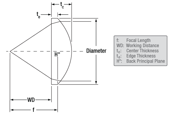
Reference Drawing for Aspheric Lens. Please note that the effective focal length is determined from the back principal plane, which does not necessarily line up with the edge of the lens.
 Zemax Files Zemax Files |
|---|
| Click on the red Document icon next to the item numbers below to access the Zemax file download. Our entire Zemax Catalog is also available. |
| Webpage Features | |
|---|---|
| Clicking this info icon below will open a window that contains specifications, performance plots, and aspheric coefficients for that specific item. | |

Features
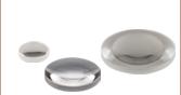
- Large Diameter Plano-Convex Aspheric Lenses
- Available in Ø12.5 mm, Ø25.0 mm, or Ø50.0 mm
- Uncoated or 245 - 420 nm Broadband AR Coating Options
- CNC Precision Polish Enables High Optical Performance
- Useful for High-Efficiency Illumination Applications
Thorlabs' Precision Aspheric Lenses are ground and polished by a computer numerical control (CNC) process. CNC polishing produces lenses with better surface irregularity, surface flatness, and focal length deviation than molded aspheric lenses. Using CNC machines, it becomes possible to produce large-diameter (≥10 mm) aspheric lenses that still provide high performance. A reference drawing for the aspheric lens is shown to the right.
The lenses sold on this page are manufactured from UV fused silica and are available in Ø12.5 mm, Ø25.0 mm, or Ø50.0 mm. Their high numerical aperture (NA) of 0.65 and low f/# ratio of 0.87 make them well suited for high-efficiency illumination applications or collimating light from a lamp, LED, or similar light source. These lenses provide a better surface quality alternative and higher transmission in the UV compared to our aspheric condenser lenses. UV fused silica provides excellent transparency deep into the UV, virtually zero autofluorescence (as measured at 193 nm), and a low coefficient of thermal expansion, making it ideal for applications from the UV to the near IR.
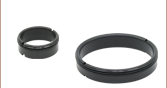
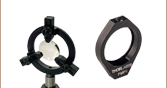
Thorlabs offers extra-thick retaining rings with SM05 (0.535"-40), SM1 (1.035"-40), and SM2 (2.035"-40) threading that provide extra clearance for spanner wrenches when mounting these lenses (see the Lens Mounting Guide tab for more information).
AR Coating Option
While our uncoated UV fused silica lenses offer excellent UV performance, improved transmission can be gained by choosing a lens with an antireflective coating. Our broadband antireflection (BBAR) UV coating provides <0.5% average reflectance per surface over 245 - 420 nm.
Optical Performance Verification
Each lens undergoes a rigorous verification procedure. Our metrology lab uses a Zygo GPI™ interferometer to generate a three-dimensional map of the lens's optical surfaces. In addition, a Taylor Hobson LUPHOScan profilometer is utilized to characterize the aspheric surface in a contact-free way. These capabilities allow us to measure and maintain our specifications with far greater confidence than would otherwise be possible. Please see the Metrology tab for more information.
Custom Aspheric Lenses
Thorlabs' CNC-polished aspheric lenses are manufactured at the production facility housed in our headquarters in Newton, NJ. Our optics business unit has a wide breadth of manufacturing capabilities that allow us to offer a variety of custom optics for both OEM sales and low quantity one-off orders. Custom lens diameters, focal lengths, substrates, coatings, and mounting options are available with prices that are comparable to our stock offerings. For more information, please see the Custom Capabilities tab or contact Tech Sales to inquire about a custom order.
Other CNC-Polished Aspheres
Thorlabs also offers CNC-polished UV fused silica aspheric lenses with lower NA, better surface quality, and tighter tolerances than those sold on this page in unmounted and mounted versions. Additional CNC-polished aspheric lenses manufactured from either N-BK7 or S-LAH64 substrate are available in unmounted and mounted versions. Available in a variety of diameters and focal lengths, these lenses are manufactured using a similar process to the high-precision lenses featured here. Please see the Selection Guide table to the right for our full selection of precision aspheric lenses.
MRF-Polished Aspheres
We also offer diffraction-limited, MRF-polished aspheres with minimal wavefront error. These lenses are free of spherical aberrations and offer the best single-element solution for many on-axis applications.
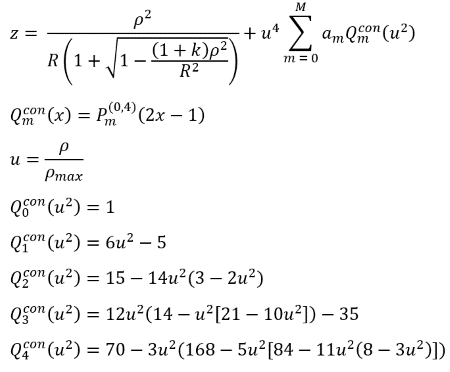
Forbes Aspheric Lens Design Formula
The lenses sold on this page were designed using the Forbes aspheric lens formula. The traditional aspheric lens formula contains a polynomial expansion that cannot be meaningfully normalized and requires many coefficients to reasonably approximate the lens surface; this polynomial set is also not orthogonal, meaning that individual terms influence each other and the total numbers of polynomial orders will affect each coefficient of the polynomial set. The Forbes aspheric lens formula, shown below, addresses these issues by introducing a new set of basis functions called Q-polynomials that are based on shifted Jacobi polynomials. Q-polynomials are a set of orthogonal polynomials describing the rotational symmetric aspherical shape. The coefficients are now normalized and the magnitude of surface form contribution is directly reflected in the coefficient itself. The first five Q-polynomial equations are defined below.
- A positive radius indicates that the center of curvature is to the right of the lens.
- A negative radius indicates that the center of curvature is to the left of the lens.

Click to Enlarge
Reference Drawing
Forbes Aspheric Lens Equation
| Definitions of Variables | |
|---|---|
| z | Sag (Surface Profile) |
| R | Radius of Curvature (mm) |
| k | Conic Constant |
| u | Normalized Aperture |
| ρmax | Maximum Semi-Aperture |
| Qconm | Shifted Jacobi Polynomials |
| am | mth Order Aspheric Coefficient |
The target values of these constants are available by clicking on the blue info icons (![]() ) below or by viewing the .pdf and .dxf files available for each lens. Links to the files can be found by clicking on the red document icon () next to each item number.
) below or by viewing the .pdf and .dxf files available for each lens. Links to the files can be found by clicking on the red document icon () next to each item number.
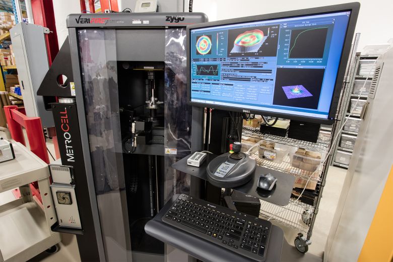
Aspheric Lens Metrology
Key Capabilities
- In Process Metrology for All CNC Polished Aspheres
- Non-Contact Interferometric and Non-Marring Profilometer Measurements
- Test Datasheets Available for OEM Sales and Custom Orders
Click to Enlarge
Zygo Verifire™ Asphere Interferometer Metrology Station
Click to Enlarge
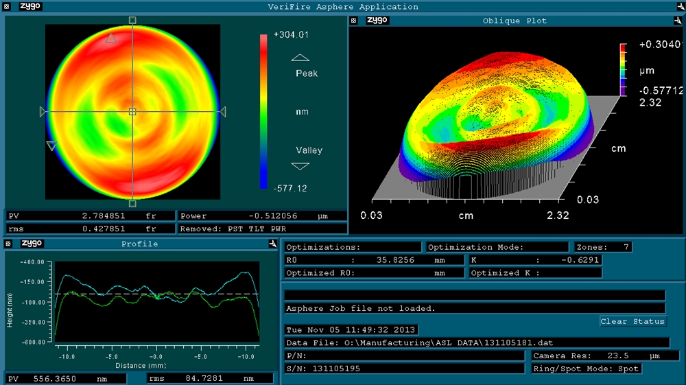
Zygo Verifire™ Asphere Interferometer Results
In order to ensure that the specifications for our CNC lenses are continuously met, we utilize a variety of advanced metrology equipment for in-process measurements of lens shape, surface roughness, and transmitted wavefront error. First, a non-contact Zygo Verifire™ Asphere Interferometer is utilized to verify the surface profile of the lenses. This instrument operates as a Fizeau interferometer by varying the distance between a reference flat or sphere (consistent with ISO 10110-12 standards) and the optic under test. Reflections from each optical surface produce an interference pattern that is recorded by the diagnostic, resulting in measurements of the low-spatial-frequency components of the aspheric surface profile. This machine is mostly used on our diffraction-limited asphere line given its superior 3D accuracy.
An example of a surface irregularity measurement performed by a Zygo Verifire™ interferometer (λ = 633 nm) is shown below. It contains interference fringes at points where the surface profile of the reference does not match the finished asphere. The relatively smooth fringe profile across the >22 mm clear aperture of the lens (shown by the lineouts in the bottom left) demonstrates the extremely low sag deviation and surface irregularity of our lenses. The lens tested here has an exceptionally low RMS surface irregularity of 0.428 fringes over its entire clear aperture and a significantly better value around the center of the lens.
Complementary measurements of each optic's high-spatial-frequency surface roughness are then made with a Zygo NewView™ white light interferometer. This device operates with a reference in one arm of the interferometer and the aspheric optic in the other. The length of one arm is varied, resulting in a white light interferogram that carries information about finer details of the optical surface. Once the surface profile of an optic has been verified, a Zygo GPI LC™ interferometer is utilized to make measurements of the transmitted wavefront error through the lens. This test ensures that the bulk of the optic is free from defects and the rear surface of the lens is flat.
To further improve our metrology capabilities, a Taylor Hobson PGI Dimension 5XL profilometer has also been added to our lens cell. This instrument makes precision contact measurements by dragging a small stylus over the surface of an optic, resulting in a complete characterization of the surface profile. This method is extremely versatile, and it can be applied to optics with a high numerical aperture or large diameter that are unsuitable for interferometric measurements. As a result, we are able to produce custom aspheric lenses with specifications that significantly exceed the capabilities of other optics manufacturers. This machine is mostly used for in process metrology of aspheric grinding.
While all machines are in use, a Taylor Hobson LUPHOScan profilometer has been utilized for the bulk of the metrology. This non-contact surface profiler uses interferometry to perform ultra-precise 3D surface measurements with high, reproducible accuracy. This machine is able to investigate our aspheres and give specific data on radius and surface irregularities due to its unique balance of speed and accuracy.
Taken together, these interferometric and contact measurements produce a complete set of three-dimensional data for each aspheric lens. This detailed quality control information allows us to manufacture the highest quality of aspheres and maintain our specifications with an extremely high degree of confidence.
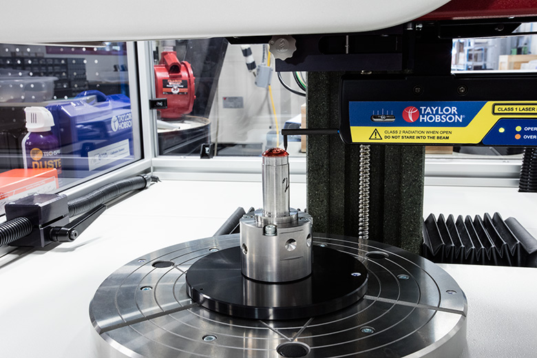
Click to Enlarge
Taylor Hobson PGI Dimension 5XL Profilometer Measuring an Aspheric Lens
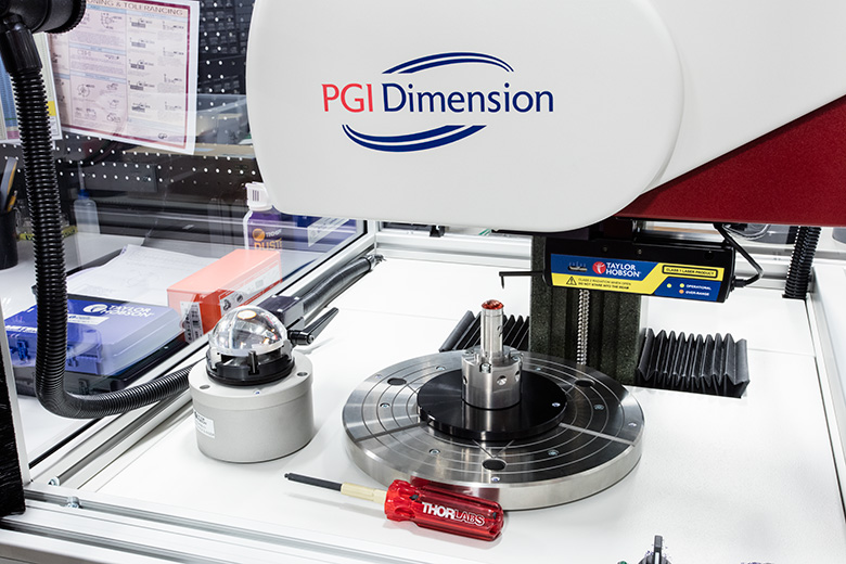
Click to Enlarge
A Taylor Hobson PGI Dimension 5XL Profilometer allows for the production of large-diameter and high-numerical-aperture aspheric lenses, such as the piece to the left of the instrument.
Custom Aspheric Lenses
Key Capabilities
- Custom Lens Diameters, Focal Lengths, Substrates, Coatings, and Mounting Options
- Enhanced Specifications and Tighter Tolerances than Stock Optics
- Support for OEM Sales and Low-Quantity Special Orders
Click to Enlarge
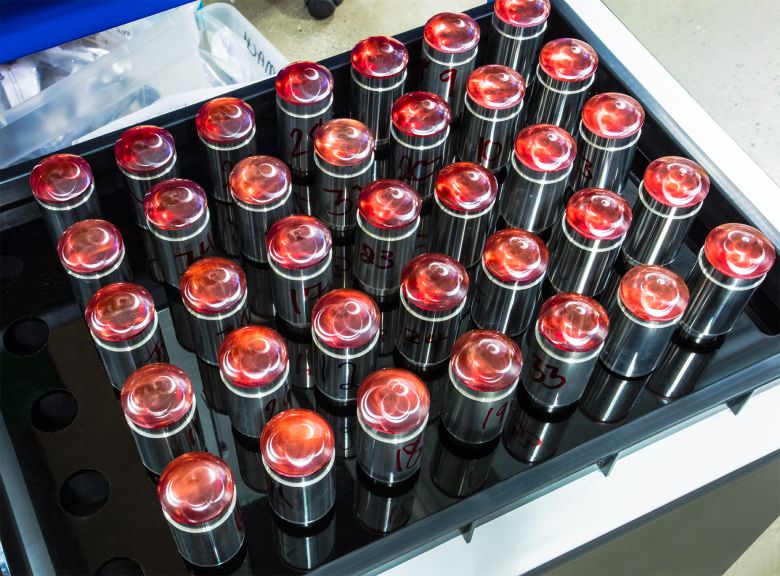
A production lot of aspheric lenses that are ready for polishing at our headquarters in Newton, NJ.
Our in-house production capabilities allow us to offer a wide variety of custom CNC-polished and MRF-polished aspheric lenses. The diameter, focal length, conjugate ratio, substrate material, and coating of these optics can all be customized to meet the unique performance requirements of a given application. In addition, custom optics can be ordered with tighter tolerances and better specifications than our stock offerings. Because of our vertically integrated manufacturing process, these custom lenses are available for both OEM sales and individual low-quantity orders.
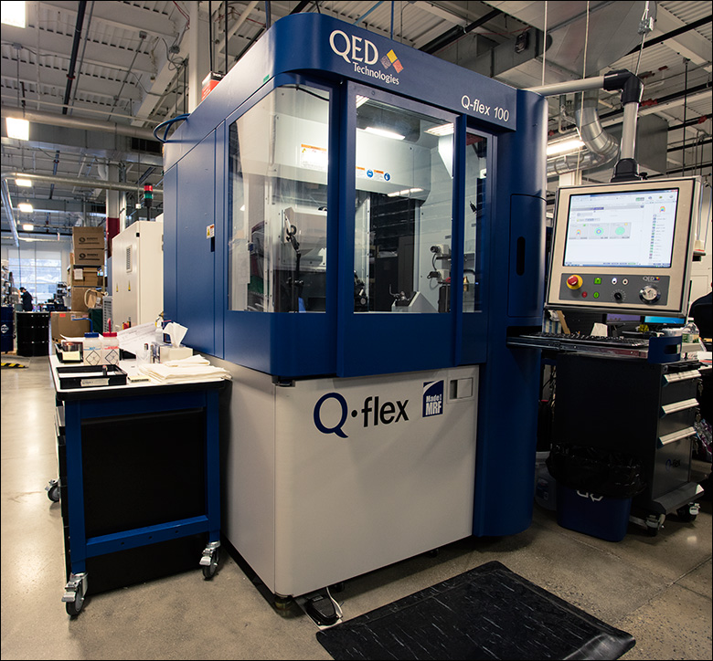
For the production of aspheric lenses, we have a CNC cell with Satisloh grinders and polishers, a QED Q-flex 100 for low wavefront error polishing, and a Satisloh C-25L for centration and custom shaping. The grinding and polishing machines allow us to manufacture both spherical and aspheric lenses with diameters from 2 mm (0.08") to 150 mm (5.91") (please contact Tech Sales with inquiries about even larger lenses). The centration machine can achieve centration down to 5 arcseconds, which is much tighter than the tolerance on most of our stock optics, and can also be used to create optics with custom shapes.
We are generally able to produce custom aspheric lenses with short lead times. For modifications to an existing part, delivery in one week is standard. For custom shapes and long focal length optics, a 6-8 week lead time is typical. To receive more information or a quote for a custom optic, please contact Tech Sales.
Click to Enlarge
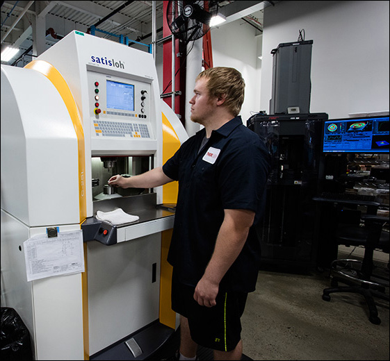
An operator loading a Satisloh Centration Machine for stock aspheric optics and custom Lens Shapes.
Click to Enlarge
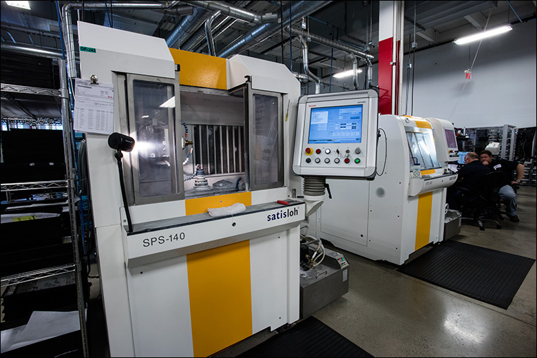
Satisloh Grinder for Aspheric Lenses
Click to Enlarge
QED Technologies Magnetorheological Finishing (MRF) Polisher
Our engineers are available to help manufacture optics for your application.
Customs are available in low quantities at prices that are comparable with our stock catalog products.
Please contact techsales@thorlabs.com with your custom optic requests.
Video 69A Mounting Standard and High-Curvature Optics in Lens Tubes
Thorlabs' retaining rings are used to secure unmounted optics within lens tubes or optic mounts. These rings are secured in position using a compatible spanner wrench. For flat or low-curvature optics, standard retaining rings manufactured from anodized aluminum are available from Ø5 mm to Ø4". For high-curvature optics, extra-thick retaining rings are available in Ø1/2", Ø1", and Ø2" sizes.
Extra-thick retaining rings offer several features that aid in mounting high-curvature optics such as aspheric lenses, short-focal-length plano-convex lenses, and condenser lenses. As seen in Video 69A, the guide flange of the spanner wrench will collide with the surface of high-curvature lenses when using a standard retaining ring, potentially scratching the optic. This contact also creates a gap between the spanner wrench and retaining ring, preventing the ring from tightening correctly. Extra-thick retaining rings provide the necessary clearance for the spanner wrench to secure the lens without coming into contact with the optic surface.
| Damage Threshold Specifications | |
|---|---|
| Coating Designation (Item # Suffix) |
Damage Threshold |
| -UV | 5.0 J/cm2 at 355 nm, 10 ns, 10 Hz, Ø0.350 mm |
Damage Threshold Data for Thorlabs' UV Fused Silica High NA Aspheres
The specifications to the right are measured data for Thorlabs' AR-Coated high NA fused silica aspheric lenses. Damage threshold specifications are constant for a given coating type, regardless of the size of the optic.
Laser Induced Damage Threshold Tutorial
The following is a general overview of how laser induced damage thresholds are measured and how the values may be utilized in determining the appropriateness of an optic for a given application. When choosing optics, it is important to understand the Laser Induced Damage Threshold (LIDT) of the optics being used. The LIDT for an optic greatly depends on the type of laser you are using. Continuous wave (CW) lasers typically cause damage from thermal effects (absorption either in the coating or in the substrate). Pulsed lasers, on the other hand, often strip electrons from the lattice structure of an optic before causing thermal damage. Note that the guideline presented here assumes room temperature operation and optics in new condition (i.e., within scratch-dig spec, surface free of contamination, etc.). Because dust or other particles on the surface of an optic can cause damage at lower thresholds, we recommend keeping surfaces clean and free of debris. For more information on cleaning optics, please see our Optics Cleaning tutorial.
Testing Method
Thorlabs' LIDT testing is done in compliance with ISO/DIS 11254 and ISO 21254 specifications.
First, a low-power/energy beam is directed to the optic under test. The optic is exposed in 10 locations to this laser beam for 30 seconds (CW) or for a number of pulses (pulse repetition frequency specified). After exposure, the optic is examined by a microscope (~100X magnification) for any visible damage. The number of locations that are damaged at a particular power/energy level is recorded. Next, the power/energy is either increased or decreased and the optic is exposed at 10 new locations. This process is repeated until damage is observed. The damage threshold is then assigned to be the highest power/energy that the optic can withstand without causing damage. A histogram such as that below represents the testing of one BB1-E02 mirror.
The photograph above is a protected aluminum-coated mirror after LIDT testing. In this particular test, it handled 0.43 J/cm2 (1064 nm, 10 ns pulse, 10 Hz, Ø1.000 mm) before damage.
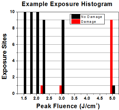
| Example Test Data | |||
|---|---|---|---|
| Fluence | # of Tested Locations | Locations with Damage | Locations Without Damage |
| 1.50 J/cm2 | 10 | 0 | 10 |
| 1.75 J/cm2 | 10 | 0 | 10 |
| 2.00 J/cm2 | 10 | 0 | 10 |
| 2.25 J/cm2 | 10 | 1 | 9 |
| 3.00 J/cm2 | 10 | 1 | 9 |
| 5.00 J/cm2 | 10 | 9 | 1 |
According to the test, the damage threshold of the mirror was 2.00 J/cm2 (532 nm, 10 ns pulse, 10 Hz, Ø0.803 mm). Please keep in mind that these tests are performed on clean optics, as dirt and contamination can significantly lower the damage threshold of a component. While the test results are only representative of one coating run, Thorlabs specifies damage threshold values that account for coating variances.
Continuous Wave and Long-Pulse Lasers
When an optic is damaged by a continuous wave (CW) laser, it is usually due to the melting of the surface as a result of absorbing the laser's energy or damage to the optical coating (antireflection) [1]. Pulsed lasers with pulse lengths longer than 1 µs can be treated as CW lasers for LIDT discussions.
When pulse lengths are between 1 ns and 1 µs, laser-induced damage can occur either because of absorption or a dielectric breakdown (therefore, a user must check both CW and pulsed LIDT). Absorption is either due to an intrinsic property of the optic or due to surface irregularities; thus LIDT values are only valid for optics meeting or exceeding the surface quality specifications given by a manufacturer. While many optics can handle high power CW lasers, cemented (e.g., achromatic doublets) or highly absorptive (e.g., ND filters) optics tend to have lower CW damage thresholds. These lower thresholds are due to absorption or scattering in the cement or metal coating.

LIDT in linear power density vs. pulse length and spot size. For long pulses to CW, linear power density becomes a constant with spot size. This graph was obtained from [1].
Pulsed lasers with high pulse repetition frequencies (PRF) may behave similarly to CW beams. Unfortunately, this is highly dependent on factors such as absorption and thermal diffusivity, so there is no reliable method for determining when a high PRF laser will damage an optic due to thermal effects. For beams with a high PRF both the average and peak powers must be compared to the equivalent CW power. Additionally, for highly transparent materials, there is little to no drop in the LIDT with increasing PRF.
In order to use the specified CW damage threshold of an optic, it is necessary to know the following:
- Wavelength of your laser
- Beam diameter of your beam (1/e2)
- Approximate intensity profile of your beam (e.g., Gaussian)
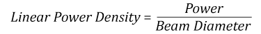
- Linear power density of your beam (total power divided by 1/e2 beam diameter)
Thorlabs expresses LIDT for CW lasers as a linear power density measured in W/cm. In this regime, the LIDT given as a linear power density can be applied to any beam diameter; one does not need to compute an adjusted LIDT to adjust for changes in spot size, as demonstrated by the graph to the right. Average linear power density can be calculated using the equation below.
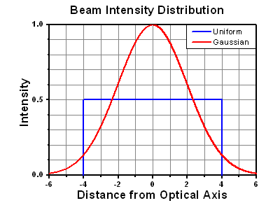
The calculation above assumes a uniform beam intensity profile. You must now consider hotspots in the beam or other non-uniform intensity profiles and roughly calculate a maximum power density. For reference, a Gaussian beam typically has a maximum power density that is twice that of the uniform beam (see lower right).
Now compare the maximum power density to that which is specified as the LIDT for the optic. If the optic was tested at a wavelength other than your operating wavelength, the damage threshold must be scaled appropriately. A good rule of thumb is that the damage threshold has a linear relationship with wavelength such that as you move to shorter wavelengths, the damage threshold decreases (i.e., a LIDT of 10 W/cm at 1310 nm scales to 5 W/cm at 655 nm):
While this rule of thumb provides a general trend, it is not a quantitative analysis of LIDT vs wavelength. In CW applications, for instance, damage scales more strongly with absorption in the coating and substrate, which does not necessarily scale well with wavelength. While the above procedure provides a good rule of thumb for LIDT values, please contact Tech Support if your wavelength is different from the specified LIDT wavelength. If your power density is less than the adjusted LIDT of the optic, then the optic should work for your application.
Please note that we have a buffer built in between the specified damage thresholds online and the tests which we have done, which accommodates variation between batches. Upon request, we can provide individual test information and a testing certificate. The damage analysis will be carried out on a similar optic (customer's optic will not be damaged). Testing may result in additional costs or lead times. Contact Tech Support for more information.
Pulsed Lasers
As previously stated, pulsed lasers typically induce a different type of damage to the optic than CW lasers. Pulsed lasers often do not heat the optic enough to damage it; instead, pulsed lasers produce strong electric fields capable of inducing dielectric breakdown in the material. Unfortunately, it can be very difficult to compare the LIDT specification of an optic to your laser. There are multiple regimes in which a pulsed laser can damage an optic and this is based on the laser's pulse length. The highlighted columns in the table below outline the relevant pulse lengths for our specified LIDT values.
Pulses shorter than 10-9 s cannot be compared to our specified LIDT values with much reliability. In this ultra-short-pulse regime various mechanics, such as multiphoton-avalanche ionization, take over as the predominate damage mechanism [2]. In contrast, pulses between 10-7 s and 10-4 s may cause damage to an optic either because of dielectric breakdown or thermal effects. This means that both CW and pulsed damage thresholds must be compared to the laser beam to determine whether the optic is suitable for your application.
| Pulse Duration | t < 10-9 s | 10-9 < t < 10-7 s | 10-7 < t < 10-4 s | t > 10-4 s |
|---|---|---|---|---|
| Damage Mechanism | Avalanche Ionization | Dielectric Breakdown | Dielectric Breakdown or Thermal | Thermal |
| Relevant Damage Specification | No Comparison (See Above) | Pulsed | Pulsed and CW | CW |
When comparing an LIDT specified for a pulsed laser to your laser, it is essential to know the following:
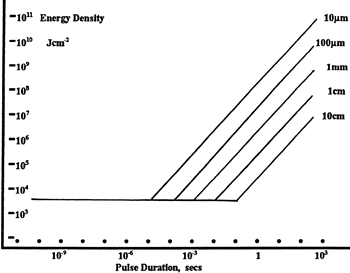
LIDT in energy density vs. pulse length and spot size. For short pulses, energy density becomes a constant with spot size. This graph was obtained from [1].
- Wavelength of your laser
- Energy density of your beam (total energy divided by 1/e2 area)
- Pulse length of your laser
- Pulse repetition frequency (prf) of your laser
- Beam diameter of your laser (1/e2 )
- Approximate intensity profile of your beam (e.g., Gaussian)
The energy density of your beam should be calculated in terms of J/cm2. The graph to the right shows why expressing the LIDT as an energy density provides the best metric for short pulse sources. In this regime, the LIDT given as an energy density can be applied to any beam diameter; one does not need to compute an adjusted LIDT to adjust for changes in spot size. This calculation assumes a uniform beam intensity profile. You must now adjust this energy density to account for hotspots or other nonuniform intensity profiles and roughly calculate a maximum energy density. For reference a Gaussian beam typically has a maximum energy density that is twice that of the 1/e2 beam.
Now compare the maximum energy density to that which is specified as the LIDT for the optic. If the optic was tested at a wavelength other than your operating wavelength, the damage threshold must be scaled appropriately [3]. A good rule of thumb is that the damage threshold has an inverse square root relationship with wavelength such that as you move to shorter wavelengths, the damage threshold decreases (i.e., a LIDT of 1 J/cm2 at 1064 nm scales to 0.7 J/cm2 at 532 nm):
You now have a wavelength-adjusted energy density, which you will use in the following step.
Beam diameter is also important to know when comparing damage thresholds. While the LIDT, when expressed in units of J/cm², scales independently of spot size; large beam sizes are more likely to illuminate a larger number of defects which can lead to greater variances in the LIDT [4]. For data presented here, a <1 mm beam size was used to measure the LIDT. For beams sizes greater than 5 mm, the LIDT (J/cm2) will not scale independently of beam diameter due to the larger size beam exposing more defects.
The pulse length must now be compensated for. The longer the pulse duration, the more energy the optic can handle. For pulse widths between 1 - 100 ns, an approximation is as follows:
Use this formula to calculate the Adjusted LIDT for an optic based on your pulse length. If your maximum energy density is less than this adjusted LIDT maximum energy density, then the optic should be suitable for your application. Keep in mind that this calculation is only used for pulses between 10-9 s and 10-7 s. For pulses between 10-7 s and 10-4 s, the CW LIDT must also be checked before deeming the optic appropriate for your application.
Please note that we have a buffer built in between the specified damage thresholds online and the tests which we have done, which accommodates variation between batches. Upon request, we can provide individual test information and a testing certificate. Contact Tech Support for more information.
[1] R. M. Wood, Optics and Laser Tech. 29, 517 (1998).
[2] Roger M. Wood, Laser-Induced Damage of Optical Materials (Institute of Physics Publishing, Philadelphia, PA, 2003).
[3] C. W. Carr et al., Phys. Rev. Lett. 91, 127402 (2003).
[4] N. Bloembergen, Appl. Opt. 12, 661 (1973).

In order to illustrate the process of determining whether a given laser system will damage an optic, a number of example calculations of laser induced damage threshold are given below. For assistance with performing similar calculations, we provide a spreadsheet calculator that can be downloaded by clicking the LIDT Calculator button. To use the calculator, enter the specified LIDT value of the optic under consideration and the relevant parameters of your laser system in the green boxes. The spreadsheet will then calculate a linear power density for CW and pulsed systems, as well as an energy density value for pulsed systems. These values are used to calculate adjusted, scaled LIDT values for the optics based on accepted scaling laws. This calculator assumes a Gaussian beam profile, so a correction factor must be introduced for other beam shapes (uniform, etc.). The LIDT scaling laws are determined from empirical relationships; their accuracy is not guaranteed. Remember that absorption by optics or coatings can significantly reduce LIDT in some spectral regions. These LIDT values are not valid for ultrashort pulses less than one nanosecond in duration.
Figure 71A A Gaussian beam profile has about twice the maximum intensity of a uniform beam profile.
CW Laser Example
Suppose that a CW laser system at 1319 nm produces a 0.5 W Gaussian beam that has a 1/e2 diameter of 10 mm. A naive calculation of the average linear power density of this beam would yield a value of 0.5 W/cm, given by the total power divided by the beam diameter:
However, the maximum power density of a Gaussian beam is about twice the maximum power density of a uniform beam, as shown in Figure 71A. Therefore, a more accurate determination of the maximum linear power density of the system is 1 W/cm.
An AC127-030-C achromatic doublet lens has a specified CW LIDT of 350 W/cm, as tested at 1550 nm. CW damage threshold values typically scale directly with the wavelength of the laser source, so this yields an adjusted LIDT value:
The adjusted LIDT value of 350 W/cm x (1319 nm / 1550 nm) = 298 W/cm is significantly higher than the calculated maximum linear power density of the laser system, so it would be safe to use this doublet lens for this application.
Pulsed Nanosecond Laser Example: Scaling for Different Pulse Durations
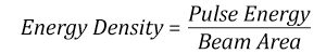
Suppose that a pulsed Nd:YAG laser system is frequency tripled to produce a 10 Hz output, consisting of 2 ns output pulses at 355 nm, each with 1 J of energy, in a Gaussian beam with a 1.9 cm beam diameter (1/e2). The average energy density of each pulse is found by dividing the pulse energy by the beam area:
As described above, the maximum energy density of a Gaussian beam is about twice the average energy density. So, the maximum energy density of this beam is ~0.7 J/cm2.
The energy density of the beam can be compared to the LIDT values of 1 J/cm2 and 3.5 J/cm2 for a BB1-E01 broadband dielectric mirror and an NB1-K08 Nd:YAG laser line mirror, respectively. Both of these LIDT values, while measured at 355 nm, were determined with a 10 ns pulsed laser at 10 Hz. Therefore, an adjustment must be applied for the shorter pulse duration of the system under consideration. As described on the previous tab, LIDT values in the nanosecond pulse regime scale with the square root of the laser pulse duration:
This adjustment factor results in LIDT values of 0.45 J/cm2 for the BB1-E01 broadband mirror and 1.6 J/cm2 for the Nd:YAG laser line mirror, which are to be compared with the 0.7 J/cm2 maximum energy density of the beam. While the broadband mirror would likely be damaged by the laser, the more specialized laser line mirror is appropriate for use with this system.
Pulsed Nanosecond Laser Example: Scaling for Different Wavelengths
Suppose that a pulsed laser system emits 10 ns pulses at 2.5 Hz, each with 100 mJ of energy at 1064 nm in a 16 mm diameter beam (1/e2) that must be attenuated with a neutral density filter. For a Gaussian output, these specifications result in a maximum energy density of 0.1 J/cm2. The damage threshold of an NDUV10A Ø25 mm, OD 1.0, reflective neutral density filter is 0.05 J/cm2 for 10 ns pulses at 355 nm, while the damage threshold of the similar NE10A absorptive filter is 10 J/cm2 for 10 ns pulses at 532 nm. As described on the previous tab, the LIDT value of an optic scales with the square root of the wavelength in the nanosecond pulse regime:
This scaling gives adjusted LIDT values of 0.08 J/cm2 for the reflective filter and 14 J/cm2 for the absorptive filter. In this case, the absorptive filter is the best choice in order to avoid optical damage.
Pulsed Microsecond Laser Example
Consider a laser system that produces 1 µs pulses, each containing 150 µJ of energy at a repetition rate of 50 kHz, resulting in a relatively high duty cycle of 5%. This system falls somewhere between the regimes of CW and pulsed laser induced damage, and could potentially damage an optic by mechanisms associated with either regime. As a result, both CW and pulsed LIDT values must be compared to the properties of the laser system to ensure safe operation.
If this relatively long-pulse laser emits a Gaussian 12.7 mm diameter beam (1/e2) at 980 nm, then the resulting output has a linear power density of 5.9 W/cm and an energy density of 1.2 x 10⁻⁴ J/cm2 per pulse. This can be compared to the LIDT values for a WPQ10E-980 polymer zero-order quarter-wave plate, which are 5 W/cm for CW radiation at 810 nm and 5 J/cm2 for a 10 ns pulse at 810 nm. As before, the CW LIDT of the optic scales linearly with the laser wavelength, resulting in an adjusted CW value of 6 W/cm at 980 nm. On the other hand, the pulsed LIDT scales with the square root of the laser wavelength and the square root of the pulse duration, resulting in an adjusted value of 55 J/cm2 for a 1 µs pulse at 980 nm. The pulsed LIDT of the optic is significantly greater than the energy density of the laser pulse, so individual pulses will not damage the wave plate. However, the large average linear power density of the laser system may cause thermal damage to the optic, much like a high-power CW beam.
| Posted Comments: | |
Ruizhe Lyu
(posted 2022-08-26 17:01:43.207) Dear Sir/Madam,
I would like to ask about the product ASL1210:
1. Is the uncoated lens appliable to 905nm? If it is, how much it is to add a B-coating.
2. If the lens is not appliable to 905nm, how much does it cost to order lens with the same modle with B-coating, but made from BK7 or similar glass.
Looking forward to hearing from you. ksosnowski
(posted 2022-08-30 04:23:46.0) Thanks for reaching out to Thorlabs. ASL1210 can be used at 905nm with roughly .33mm focal shift and with similar transmission to the visible spectrum. Some of the other specs will shift slightly at this wavelength as well. The AL1210-B is our closest alternative, using S-LAH64 and with NA=0.55, and there would be less than 0.1mm focal shift from the 780nm design wavelength. I have reached out directly to discuss this application further. |
| Item # | Info | OD | EFLb | WDb,c | Clear Aperturea | tc | te | |
|---|---|---|---|---|---|---|---|---|
| Collimation (Aspheric Side) |
Focusing (Plano Side) |
|||||||
| ASL1210 | 12.5 mm | 10.0 mm | 4.9 mm | Ø11.43 mm | Ø8.4 mm | 7.50 mm | 1.9 mm | |
| ASL2520 | 25.00 mm | 20.0 mm | 9.9 mm | Ø22.86 mm | Ø17.4 mm | 14.90 mm | 3.6 mm | |
| ASL5040 | 50.00 mm | 40.0 mm | 19.7 mm | Ø45.72 mm | Ø35.1 mm | 29.85 mm | 7.3 mm | |
| Item # | Info | OD | EFLb | WDb,c | Clear Aperturea | tc | te | AR Coating |
|
|---|---|---|---|---|---|---|---|---|---|
| Collimation (Aspheric Side) |
Focusing (Plano Side) |
||||||||
| ASL1210-UV | 12.5 mm | 10.0 mm | 4.9 mm | Ø11.43 mm | Ø8.4 mm | 7.50 mm | 1.9 mm | 245 - 420 nm Ravg < 0.5% Tavg > 96.5% 0°±5° AOI |
|
| ASL2520-UV | 25.0 mm | 20.0 mm | 9.9 mm | Ø22.86 mm | Ø17.4 mm | 14.90 mm | 3.6 mm | ||
| ASL5040-UV | 50.0 mm | 40.0 mm | 19.7 mm | Ø45.72 mm | Ø35.1 mm | 29.85 mm | 7.3 mm | ||