 Products Home
Zoom Fiber Collimators
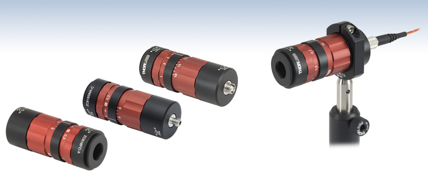
- Adjustable Focal Length: 6 - 18 mm
- FC/PC, FC/APC, or SMA Connector
- Three AR Coating Options
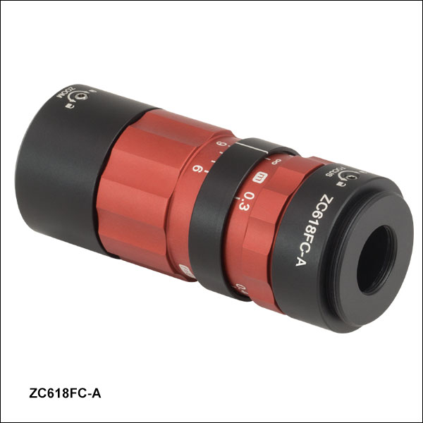
ZC618FC-A
FC/PC Connector,
AR Coated for
400 - 650 nm
ZC618SMA-C
SMA Connector,
AR Coated for
1050 - 1650 nm
Application Idea
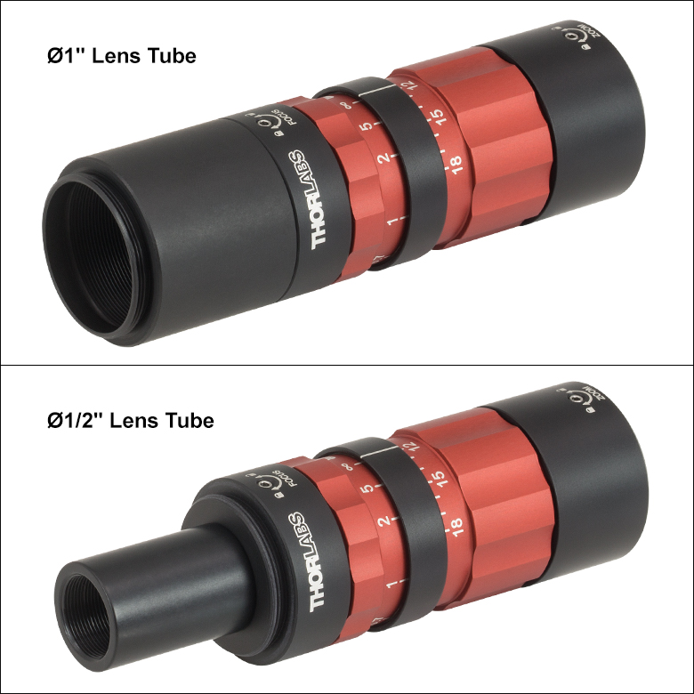
Zoom Fiber Collimator Mounted in a Ø1" Lens Tube Slip Ring (SM1RC)
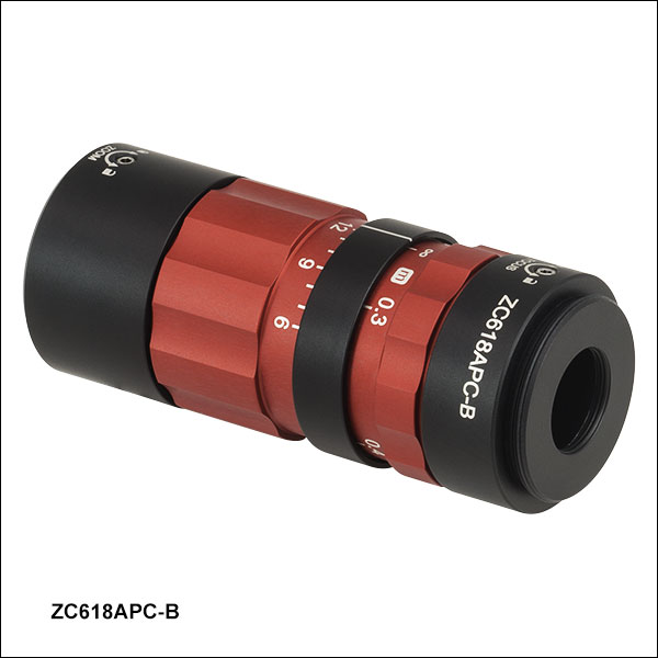
ZC618APC-B
FC/APC Connector,
AR Coated for
650 - 1050 nm


Please Wait
| Mounting Solutions | ||
|---|---|---|
| Item # | Description | Threads/Bores |
| SM2A21 | Ø2" Mounting Adapter | SM2 (2.035"-40) External Threads |
| SM1RC (SM1RC/M) |
Ø1" (SM1) Slim Lens Tube Slip Ring |
Post Mountable via 8-32 (M4) Mounting Hole |
| SM1TC | Ø1" (SM1) Slim Lens Tube Clamp | Post Mountable via #8 (M4) Counterbore |
| CP36 | 30 mm Cage Plate, Ø1.2" Central Double Bore |
4 Through Holes at Corners for ER Series Cage Rods |
Click to Enlarge
The end of the zoom fiber collimator has internal SM05 threading and external SM1 threading for attaching Ø1/2" and Ø1" lens tubes.
Features
- Focal Length Adjustable Between 6 mm and 18 mm
- Three Broadband Antireflection Coatings Available (See the Coating Tab for Plots)
- A-Coating: Rmax < 0.5% for 400 nm - 650 nm
- B-Coating: Rmax < 0.5% for 650 nm - 1050 nm
- C-Coating: Rmax < 0.5% for 1050 nm - 1650 nm
- Closest Focusing Distance: 0.3 m
- Nearly Gaussian Output from Single Mode Fiber
- Maximum NA: 0.25
- Low Wavefront Error: λ/10 Typical (P-V at 633 nm for Fiber NA = 0.14)
- Pointing Stability During Zooming:
- FC/PC and FC/APC: <1 mrad
- SMA905: <4 mrad
- Available With an FC/PC, FC/APC, or SMA905 Connector
- Fits Inside Any Ø1.2" Mount (See Table at Right for Options)
- Excellent Off-Axis Performance for Large Multimode Fibers (See the Multimode Tab)
- Compatible with SM05/SM1 Lens Tubes
- Can be Used as a Coupler or Collimator
Thorlabs' Zoom Fiber Collimators provide a variable focal length between 6 mm and 18 mm, while maintaining the collimation of the beam. As a result, the size of the beam can be changed without altering the collimation (see the Performance tab for a video). In addition to the zooming capability, the divergence of the collimated beam can be finely adjusted or the beam can be focused anywhere between the maximum waist distance and the closest focusing distance of 0.3 m, allowing one to easily maximize the coupling efficiency of a free-space laser beam into a fiber. See the Performance tab for more information about adjusting the focusing and zoom. This universal device can be utilized in a broad range of applications, saving time previously spent searching for the best suited fixed fiber collimator.
These zoom collimators incorporate an air-spaced lens design, resulting in superior beam quality compared to that offered by aspheric lens collimators. The benefits of the low-aberration air-spaced design include an M2 term closer to 1 (Gaussian) and less wavefront error.
Our zoom collimators are available from stock with AR coatings for three different wavelength ranges (400 nm - 650 nm, 650 nm - 1050 nm, or 1050 nm - 1650 nm) and with either an FC/PC, FC/APC, or SMA connector. The broadband AR coating is deposited on both surfaces of each lens in the collimator (see the Coating tab for details) in order to minimize losses caused by surface reflections. Please contact Technical Support if you are interested in zoom collimators with a V-coating centered at a specific wavelength.
We also offer a line of fixed triplet fiber collimators; aspheric fiber collimators, including our fixed collimators; and our FiberPort adjustable collimation packages that are well suited for use with a wide range of wavelengths. For our complete line of collimation and coupling options, please see the Collimator Guide tab.
Mounting Options
The output end of the zoom collimator is equipped with both internal SM05 (0.535"-40) and external SM1 (1.035"-40) threading, which makes it easy to integrate these zoom collimators into our entire line of optomechanical components. The threaded ring at the end of the zoom collimator does not rotate when turning the zoom or focus adjustment rings, allowing the user to adjust the beam size without disturbing any attached optics, thus maintaining pointing stability (see the Performance tab for more information).
The zoom collimator has a diameter of 1.2" (30.5 mm), which is identical to Thorlabs' SM1 Lens Tubes. The three black rings, located on both ends and between the zoom and focus adjustment rings, are provided for mounting the zoom collimator to a post via our SM1RC or SM1RC/M Lens Tube Slip Ring or SM1TC Lens Tube Clamp. These collimators can also be inserted into a 30 mm cage system using a CP36 Cage Plate. Alternatively, the SM2A21 adapter can be used to convert the mounting ring outer diameter to 2", making it compatible with Thorlabs' SM2 Lens Tubes, 60 mm Cage Systems, and Ø2" optic mounts.
| Specifications | |||||||||
|---|---|---|---|---|---|---|---|---|---|
| Item # | ZC618APC-A | ZC618FC-A | ZC618SMA-A | ZC618APC-B | ZC618FC-B | ZC618SMA-B | ZC618APC-C | ZC618FC-C | ZC618SMA-C |
| Connector Style | 2.2 mm Wide Key FC/APC |
2.2 mm Wide Key FC/PC |
SMA905 | 2.2 mm Wide Key FC/APC |
2.2 mm Wide Key FC/PC |
SMA905 | 2.2 mm Wide Key FC/APC |
2.2 mm Wide Key FC/PC |
SMA905 |
| AR Coating Range | 400 - 650 nm | 650 - 1050 nm | 1050 - 1650 nm | ||||||
| Transmission at Selected Laser Lines |
80% at 405 nm 87% at 543 nm 90% at 633 nm |
89% at 780 nm 92% at 980 nm |
91% at 1064 nm 88% at 1310 nm 84% at 1550 nm |
||||||
| Typical Collimated Beam Diametera,b |
1.06 - 3.50 mm (SM400 at 405 nm) 1.08 - 3.49 mm (SM450 at 543 nm) 1.08 - 3.39 mm (SM600 at 633 nm) |
1.24 - 3.90 mm (780HP at 780 nm) 1.27 - 3.89 mm (SM980-5.8-125 at 980 nm) |
1.24 - 3.92 mm (SM980-5.8-125 at 1064 nm) 1.07 - 3.27 mm (SMF-28-J9 at 1310 nm) 1.10 - 3.30 mm (SMF-28-J9 at 1550 nm) |
||||||
| Reflectance | Rmax < 0.5% | ||||||||
| Effective Focal Length | 6 - 18 mm | ||||||||
| Maximum Fiber NA | 0.25 | ||||||||
| Closest Focusing Distance | 0.3 m | ||||||||
| Pointing Stability During Zooming | <1 mrad | <4 mrad | <1 mrad | <4 mrad | <1 mrad | <4 mrad | |||
| Damage Threshold Specificationsc | ||
|---|---|---|
| Item # Suffix | AR Coating | Damage Threshold |
| -A | 400 - 650 nm | 3 J/cm2 (532 nm, 10 Hz, 10 ns, Ø408 μm) |
| -B | 650 - 1050 nm | 7.5 J/cm2 (810 nm, 10 Hz, 10 ns, Ø76.9 μm) |
| -C | 1050 - 1650 nm | 3 J/cm2 (1542 nm, 1 Hz, 10 ns, Ø268 μm) |
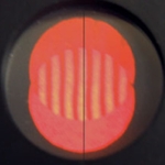
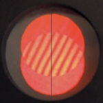
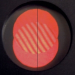
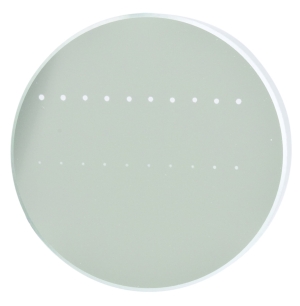
The interference fringes produced by the shearing interferometer (SI035 with a mounted viewing screen system SIVS) remain parallel to the reference line as the size of the beam changes by adjusting the focal length of the zoom fiber collimator. For more information on how a shearing interferometer works, please see our full presentation here.
Collimation
Thorlabs' Shearing Interferometers can be used to determine if a coherent beam of light is collimated. The design consists of a wedged optical flat mounted at 45° and a diffuser plate with a ruled reference line down the middle. These interferometers are designed to provide qualitative analysis of a beam's collimation.
The diffuser plate is used to view the interference fringes created by Fresnel reflections from the front and back surfaces of the optical flat. If the beam is collimated, the resulting fringe pattern will be parallel to the ruled reference line. In addition to the degree of collimation, the fringes will also be sensitive to spherical aberration, coma, and astigmatism.
The video to the right shows the output of a shearing interferometer as the focal length is adjusted on a zoom fiber collimator. The fringes remain parallel to the reference line, meaning that the beam remains collimated as the size of the beam is adjusted (see images below for a reference).
Pointing Stability
The tightly toleranced wide key FC/PC and FC/APC receptacle and ceramic sleeve yield high pointing repeatability by allowing the user to easily remove and replace the fiber. The fact that the lenses in these collimators slide within the housing rather than rotating results in superior pointing stability (<1 mrad). The SMA receptacle and metal ferrule also produces an excellent pointing stability (<4 mrad).
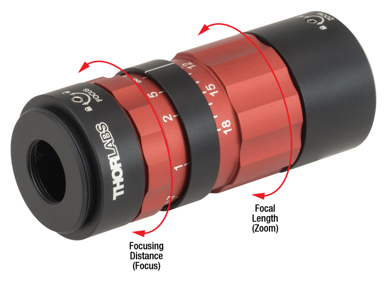
Adjustment
Light collimated from a single mode fiber has a nearly Gaussian beam profile, with waist diameter and divergence angle depending on both the wavelength of light and the mode field diameter (MFD) of the fiber, in addition to the focal length of the collimator. When our Zoom Fiber Collimators are adjusted so that they do not fully collimate the beam, the position of the beam waist will also exhibit sensitivity to the wavelength and MFD. In light of these application-specific dependencies, the ring has been engraved with the focusing distances obtained for light from a point source at the fiber tip location, using ray optics. These wavelength-independent values do not correspond to the waist locations for beams obtained from single mode fibers, so if the waist location is important for a given application then it should be determined in the particular setup.
Thorlabs' zoom fiber collimators provide a variable focal length between 6 and 18 mm, while maintaining the collimation of the beam. In addition, the divergence of the collimated beam can be finely adjusted or the beam can be focused between the maximum waist distance (see the Divergence tab) to the closest focusing distance of 0.3 m, allowing the coupling efficiency of a free-space laser beam into a fiber to be easily maximized.
The image to the right illustrates the two ways to adjust the collimator. To adjust the focusing distance, rotate the red section of the housing farthest from the fiber connector. This will effectively alter the focus of the beam. To adjust the focal length, rotate the red section closest to the fiber connector. This will effectively alter the size of the beam.
There are setscrews on each end for locking the zoom, focus, or both with the included 0.05" (1.3 mm) hex key.
Longitudinal Chromatic Aberration
When used within the specified operating wavelength range, these zoom fiber collimators are designed to minimize the longitudinal chromatic aberration over the entire range of focal length adjustment. Longitudinal chromatic aberration occurs when the focal planes for different wavelengths of light are located at different distances from the same focusing optic.
The longitudinal aberration produced by the fiber zoom collimators when they are used to couple free-space collimated beams into fibers is shown the graphs below. The theoretical deviation of the focal plane location from the nominal focal length [i.e., the number indicated by the focal length adjustment (zoom) ring] is plotted over the operating wavelength range. The calculation was performed for each coating type at focal length settings of 6 mm, 12 mm, and 18 mm (i.e., the focal length for each data set would be set by turning only the red ring closest to the fiber connector).
Click to Enlarge
Click Here for Theoretical Data
The longitudinal chromatic aberration for the ZC618FC-A, ZC618APC-A, and ZC618SMA-A zoom fiber collimators used as a coupler with the focal length set at 6 mm, 12 mm, and 18 mm. The blue-shaded region indicates the specified operating wavelength range of the collimator.

Click to Enlarge
Click Here for Theoretical Data
The longitudinal chromatic aberration for the ZC618FC-B, ZC618APC-B, and ZC618SMA-B zoom fiber collimators used as a coupler with the focal length set at 6 mm, 12 mm, and 18 mm. The blue-shaded region indicates the specified operating wavelength range of the collimator.
Click to Enlarge
Click Here for Theoretical Data
The longitudinal chromatic aberration for the ZC618FC-C, ZC618APC-C, and ZC618SMA-C zoom fiber collimators used as a coupler with the focal length set at 6 mm, 12 mm, and 18 mm. The blue-shaded region indicates the specified operating wavelength range of the collimator.
The graphs below illustrate the theoretical 1/e2 beam diameter as a function of propagation distance for certain single mode-coupled laser wavelengths using our Zoom Fiber Collimators, adjusted for minimum divergence by setting the focusing distance to infinity. Beam diameter data are shown for eight common wavelengths and three collimator focal length settings. The effect of changing the fiber, wavelength, or focal length can be estimated using the theoretical approximations below the graphs.

Click to Enlarge
Click Here for Theoretical Data
This data is calculated for SM400 single mode fiber and our zoom collimators for 400 - 650 nm.
Click to Enlarge
Click Here for Theoretical Data
This data is calculated for SM450 single mode fiber and our zoom collimators for 400 - 650 nm.
Click to Enlarge
Click Here for Theoretical Data
This data is calculated for SM600 single mode fiber and our zoom collimators for 400 - 650 nm.
Click to Enlarge
Click Here for Theoretical Data
This data is calculated for 780HP single mode fiber and our zoom collimators for 650 - 1050 nm.
Click to Enlarge
Click Here for Theoretical Data
This data is calculated for SM980-5.8-125 single mode fiber and our zoom collimators for 650 - 1050 nm.
Click to Enlarge
Click Here for Theoretical Data
This data is calculated for SM980-5.8-125 single mode fiber and our zoom collimators for 1050 - 1650 nm.

Click to Enlarge
Click Here for Theoretical Data
This data is calculated for SMF-28-J9 single mode fiber and our zoom collimators for 1050 - 1650 nm.
Click to Enlarge
Click Here for Theoretical Data
This data is calculated for SMF-28-J9 single mode fiber and our zoom collimators for 1050 - 1650 nm.
Theoretical Approximation of the Divergence Angle
The divergence angle can be approximated theoretically using the formula below as long as the light emerging from the fiber has a Gaussian intensity profile. Consequently, the formula works well for single mode fibers, but it will underestimate the divergence angle for multimode (MM) fibers since the light emerging from a MM fiber has a non-Gaussian intensity profile.
The Full Divergence Angle (in degrees) is given by
where MFD is the mode field diameter of the fiber and f is the focal length of the collimator. MFD and f must have the same units in this equation.
Example:
When the ZC618APC-A collimator is used with a single mode fiber patch cable, such as our P3-460B-FC-1 such that MFD = 3.6 µm, f ≈ 12.0 mm, and λ = 543 nm, the divergence angle is
θ ≈ (0.0036 mm / 12.0 mm)*(180/3.1416) ≈ 0.017° or 0.30 mrad.
Theoretical Approximation of the Output Beam Diameter
The 1/e2 output beam diameter at the front focal plane of the collimator, when the collimator is set to minimize divergence, can be found using the approximation
where λ is the wavelength of light being used, MFD is the mode field diameter of the fiber, and f is the focal length of the collimator.
Example:
When the ZC618APC-C collimator (f = 12.0 mm) is used with the P1-SMF28E-FC-1 patch cable (MFD = 10.5 µm) and 1550 nm light, the output beam diameter is
(4)(1550 nm)[12.0 mm / (π · 10.5 µm)] = 2.26 mm
Theoretical Approximation of the Maximum Waist Distance
For a given collimator, SM fiber, and wavelength of light, there is a maximum possible waist distance, which can be approximated by
where f is the focal length of the collimator, λ is the wavelength of light used, and MFD is the mode field diameter of the fiber.
Example:
When the ZC618APC-A collimator is used with a single mode fiber patch cable, such as our P3-460B-FC-1 such that MFD = 3.6 µm, f≈ 12.0 mm, and λ = 543 nm, then the maximum waist distance is
(12 mm) + (2 (12 mm)2 (543 nm) / (3.1416) (3.6 µm)2) = 3.85 m.
Off-Axis Performance
Thorlabs' FC/PC- and SMA-terminated zoom fiber collimators are excellent for use with multimode fibers. To demonstrate this feature, a ZC618SMA-A zoom fiber collimator was used to collimate light from a halogen light source with the use of a BFL105LS02 Round-to-Linear Multimode Fiber Bundle. The collimator was set up to image the fiber’s output onto a viewing screen placed approximately 1 m from the output.
The video to the right shows the focal length being varied through the entire range (18 mm to 6 mm) and back. The focus plane remains constant, always producing a sharp image of the multimode fiber, throughout this adjustment. The video also demonstrates the collimator’s excellent off-axis image performance for large multimode fiber cores, showing all 7 fiber cores in sharp, distinguishable focus.
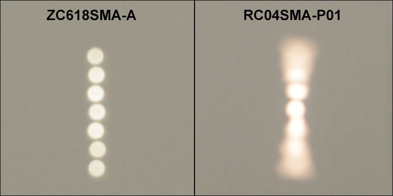
Click to Enlarge
The picture above shows the image produced by the ZC618SMA-A Zoom Fiber Collimator (left) and the RC04SMA-P01 Protected Silver Reflective Collimator (right) using a round-to-linear fiber bundle.
By contrast, when placed in the same experimental setup, the RC04SMA-P01 Reflective Collimator demonstrates significant off-axis aberrations (i.e. coma, astigmatism, and field curvature). These aberrations result from the fact that parabolic mirrors do not perfectly collimate light from point sources located away from the focus of the paraboloid. The image above shows a side by side comparison between the reflective collimator and the zoom fiber collimator.

Click to Enlarge
The drawing above is an illustration of multimode fiber core image formation. The image is formed at the focusing distance determined by the FOCUS adjustment ring.
Imaging of Multimode Fiber Cores
When the focusing distance of the collimator is finite, an image of the multimode fiber core will be produced. The drawing to the right shows a ray optics picture of the formation of an image of a multimode fiber core. As the focusing distance of the collimator is changed, the size of the image will also change. The size of the image produced can be approximated with the following equation:
 .
.
The graphs below illustrate the theoretical imaged core diameter as a function of focusing distance using our SMA- or FC/PC-terminated achromatic fiber collimators. These results are independent of wavelength and connector type.


Relative Illumination
For fibers with high NA and large cores, vignetting (reduction of a beam's intensity at the edges compared to the center) can occur. The graph to the right shows the relative intensity in the image of a fiber with a uniform output beam profile and NA of 0.25, plotted against the radial position in the core being imaged to the measured point in the image.
The graphs below show the reflectance with respect to wavelength of the AR coatings used on the 14 lens surfaces in our zoom fiber collimators (two surfaces per lens). The blue shaded region indicates the wavelength range specified for each coating. The table below details which AR coating is used with each collimator.

| Antireflection Coatings | ||||||
|---|---|---|---|---|---|---|
| Item # | Coating Code | Wavelength Range | Reflectance | |||
| ZC618APC-A | A | 400 - 650 nma | Rmax < 0.5% | |||
| ZC618FC-A | ||||||
| ZC618SMA-A | ||||||
| ZC618APC-B | B | 650 - 1050 nm | Rmax < 0.5% | |||
| ZC618FC-B | ||||||
| ZC618SMA-B | ||||||
| ZC618APC-C | C | 1050 - 1650 nm | Rmax < 0.5% | |||
| ZC618FC-C | ||||||
| ZC618SMA-C | ||||||
 Zemax Files Zemax Files |
|---|
| Click on the red Document icon next to the item numbers below to access the Zemax file download. |
The linked Zemax files are a theoretical approximation of the performance of each collimator. Performance over an extended wavelength range can be obtained by using these Zemax files. Using these black box files allows you to see how the beam profile will change as you change the focal length, the focusing distance, or as you move away from the zoom collimator. Below are screen shots of what you will see when you open the file as well as descriptions on how to change the operating wavelength. For this example, the ZC618APC-A black box file was used.

Click to Enlarge
The black box Zemax file should display this screen upon opening the file.

Click to Enlarge
The Zemax file provides five different focal lengths setup as different configurations. The distances for the Compensator and Variator lens groups are fixed by the optomechanics and should not be changed. The position of the Focusing group can be changed individually for each focal length.
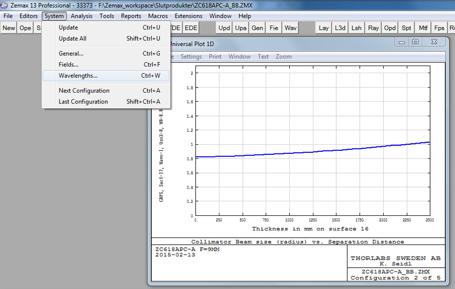
Click to Enlarge
Click on "System" in the program header bar and then select "Wavelengths".
Click to Enlarge
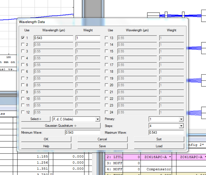
Change the current alignment wavelength, indicated by the first checkmarked row, to your operating wavelength. Click "Update" in the graph window from the previous screen.

Click to Enlarge
Change the current waist size “W0”, to the half Mode Field Diameter of your operating fiber. Click "Update" in the graph window from the previous screen.
| Damage Threshold Specifications | ||
|---|---|---|
| Item # Suffix | AR Coating | Damage Threshold |
| -A | 400 - 650 nm | 3 J/cm2 (532 nm, 10 Hz, 10 ns, Ø408 μm) |
| -B | 650 - 1050 nm | 7.5 J/cm2 (810 nm, 10 Hz, 10 ns, Ø76.9 μm) |
| -C | 1050 - 1650 nm | 3 J/cm2 (1542 nm, 1 Hz, 10 ns, Ø268 μm) |
Damage Threshold Data for Thorlabs' Zoom Fiber Collimators
The specifications to the right are measured data for Thorlabs' zoom fiber collimators.
Laser Induced Damage Threshold Tutorial
The following is a general overview of how laser induced damage thresholds are measured and how the values may be utilized in determining the appropriateness of an optic for a given application. When choosing optics, it is important to understand the Laser Induced Damage Threshold (LIDT) of the optics being used. The LIDT for an optic greatly depends on the type of laser you are using. Continuous wave (CW) lasers typically cause damage from thermal effects (absorption either in the coating or in the substrate). Pulsed lasers, on the other hand, often strip electrons from the lattice structure of an optic before causing thermal damage. Note that the guideline presented here assumes room temperature operation and optics in new condition (i.e., within scratch-dig spec, surface free of contamination, etc.). Because dust or other particles on the surface of an optic can cause damage at lower thresholds, we recommend keeping surfaces clean and free of debris. For more information on cleaning optics, please see our Optics Cleaning tutorial.
Testing Method
Thorlabs' LIDT testing is done in compliance with ISO/DIS 11254 and ISO 21254 specifications.
First, a low-power/energy beam is directed to the optic under test. The optic is exposed in 10 locations to this laser beam for 30 seconds (CW) or for a number of pulses (pulse repetition frequency specified). After exposure, the optic is examined by a microscope (~100X magnification) for any visible damage. The number of locations that are damaged at a particular power/energy level is recorded. Next, the power/energy is either increased or decreased and the optic is exposed at 10 new locations. This process is repeated until damage is observed. The damage threshold is then assigned to be the highest power/energy that the optic can withstand without causing damage. A histogram such as that below represents the testing of one BB1-E02 mirror.
The photograph above is a protected aluminum-coated mirror after LIDT testing. In this particular test, it handled 0.43 J/cm2 (1064 nm, 10 ns pulse, 10 Hz, Ø1.000 mm) before damage.
| Example Test Data | |||
|---|---|---|---|
| Fluence | # of Tested Locations | Locations with Damage | Locations Without Damage |
| 1.50 J/cm2 | 10 | 0 | 10 |
| 1.75 J/cm2 | 10 | 0 | 10 |
| 2.00 J/cm2 | 10 | 0 | 10 |
| 2.25 J/cm2 | 10 | 1 | 9 |
| 3.00 J/cm2 | 10 | 1 | 9 |
| 5.00 J/cm2 | 10 | 9 | 1 |
According to the test, the damage threshold of the mirror was 2.00 J/cm2 (532 nm, 10 ns pulse, 10 Hz, Ø0.803 mm). Please keep in mind that these tests are performed on clean optics, as dirt and contamination can significantly lower the damage threshold of a component. While the test results are only representative of one coating run, Thorlabs specifies damage threshold values that account for coating variances.
Continuous Wave and Long-Pulse Lasers
When an optic is damaged by a continuous wave (CW) laser, it is usually due to the melting of the surface as a result of absorbing the laser's energy or damage to the optical coating (antireflection) [1]. Pulsed lasers with pulse lengths longer than 1 µs can be treated as CW lasers for LIDT discussions.
When pulse lengths are between 1 ns and 1 µs, laser-induced damage can occur either because of absorption or a dielectric breakdown (therefore, a user must check both CW and pulsed LIDT). Absorption is either due to an intrinsic property of the optic or due to surface irregularities; thus LIDT values are only valid for optics meeting or exceeding the surface quality specifications given by a manufacturer. While many optics can handle high power CW lasers, cemented (e.g., achromatic doublets) or highly absorptive (e.g., ND filters) optics tend to have lower CW damage thresholds. These lower thresholds are due to absorption or scattering in the cement or metal coating.

LIDT in linear power density vs. pulse length and spot size. For long pulses to CW, linear power density becomes a constant with spot size. This graph was obtained from [1].
Pulsed lasers with high pulse repetition frequencies (PRF) may behave similarly to CW beams. Unfortunately, this is highly dependent on factors such as absorption and thermal diffusivity, so there is no reliable method for determining when a high PRF laser will damage an optic due to thermal effects. For beams with a high PRF both the average and peak powers must be compared to the equivalent CW power. Additionally, for highly transparent materials, there is little to no drop in the LIDT with increasing PRF.
In order to use the specified CW damage threshold of an optic, it is necessary to know the following:
- Wavelength of your laser
- Beam diameter of your beam (1/e2)
- Approximate intensity profile of your beam (e.g., Gaussian)
- Linear power density of your beam (total power divided by 1/e2 beam diameter)
Thorlabs expresses LIDT for CW lasers as a linear power density measured in W/cm. In this regime, the LIDT given as a linear power density can be applied to any beam diameter; one does not need to compute an adjusted LIDT to adjust for changes in spot size, as demonstrated by the graph to the right. Average linear power density can be calculated using the equation below.
The calculation above assumes a uniform beam intensity profile. You must now consider hotspots in the beam or other non-uniform intensity profiles and roughly calculate a maximum power density. For reference, a Gaussian beam typically has a maximum power density that is twice that of the uniform beam (see lower right).
Now compare the maximum power density to that which is specified as the LIDT for the optic. If the optic was tested at a wavelength other than your operating wavelength, the damage threshold must be scaled appropriately. A good rule of thumb is that the damage threshold has a linear relationship with wavelength such that as you move to shorter wavelengths, the damage threshold decreases (i.e., a LIDT of 10 W/cm at 1310 nm scales to 5 W/cm at 655 nm):
While this rule of thumb provides a general trend, it is not a quantitative analysis of LIDT vs wavelength. In CW applications, for instance, damage scales more strongly with absorption in the coating and substrate, which does not necessarily scale well with wavelength. While the above procedure provides a good rule of thumb for LIDT values, please contact Tech Support if your wavelength is different from the specified LIDT wavelength. If your power density is less than the adjusted LIDT of the optic, then the optic should work for your application.
Please note that we have a buffer built in between the specified damage thresholds online and the tests which we have done, which accommodates variation between batches. Upon request, we can provide individual test information and a testing certificate. The damage analysis will be carried out on a similar optic (customer's optic will not be damaged). Testing may result in additional costs or lead times. Contact Tech Support for more information.
Pulsed Lasers
As previously stated, pulsed lasers typically induce a different type of damage to the optic than CW lasers. Pulsed lasers often do not heat the optic enough to damage it; instead, pulsed lasers produce strong electric fields capable of inducing dielectric breakdown in the material. Unfortunately, it can be very difficult to compare the LIDT specification of an optic to your laser. There are multiple regimes in which a pulsed laser can damage an optic and this is based on the laser's pulse length. The highlighted columns in the table below outline the relevant pulse lengths for our specified LIDT values.
Pulses shorter than 10-9 s cannot be compared to our specified LIDT values with much reliability. In this ultra-short-pulse regime various mechanics, such as multiphoton-avalanche ionization, take over as the predominate damage mechanism [2]. In contrast, pulses between 10-7 s and 10-4 s may cause damage to an optic either because of dielectric breakdown or thermal effects. This means that both CW and pulsed damage thresholds must be compared to the laser beam to determine whether the optic is suitable for your application.
| Pulse Duration | t < 10-9 s | 10-9 < t < 10-7 s | 10-7 < t < 10-4 s | t > 10-4 s |
|---|---|---|---|---|
| Damage Mechanism | Avalanche Ionization | Dielectric Breakdown | Dielectric Breakdown or Thermal | Thermal |
| Relevant Damage Specification | No Comparison (See Above) | Pulsed | Pulsed and CW | CW |
When comparing an LIDT specified for a pulsed laser to your laser, it is essential to know the following:
LIDT in energy density vs. pulse length and spot size. For short pulses, energy density becomes a constant with spot size. This graph was obtained from [1].
- Wavelength of your laser
- Energy density of your beam (total energy divided by 1/e2 area)
- Pulse length of your laser
- Pulse repetition frequency (prf) of your laser
- Beam diameter of your laser (1/e2 )
- Approximate intensity profile of your beam (e.g., Gaussian)
The energy density of your beam should be calculated in terms of J/cm2. The graph to the right shows why expressing the LIDT as an energy density provides the best metric for short pulse sources. In this regime, the LIDT given as an energy density can be applied to any beam diameter; one does not need to compute an adjusted LIDT to adjust for changes in spot size. This calculation assumes a uniform beam intensity profile. You must now adjust this energy density to account for hotspots or other nonuniform intensity profiles and roughly calculate a maximum energy density. For reference a Gaussian beam typically has a maximum energy density that is twice that of the 1/e2 beam.
Now compare the maximum energy density to that which is specified as the LIDT for the optic. If the optic was tested at a wavelength other than your operating wavelength, the damage threshold must be scaled appropriately [3]. A good rule of thumb is that the damage threshold has an inverse square root relationship with wavelength such that as you move to shorter wavelengths, the damage threshold decreases (i.e., a LIDT of 1 J/cm2 at 1064 nm scales to 0.7 J/cm2 at 532 nm):
You now have a wavelength-adjusted energy density, which you will use in the following step.
Beam diameter is also important to know when comparing damage thresholds. While the LIDT, when expressed in units of J/cm², scales independently of spot size; large beam sizes are more likely to illuminate a larger number of defects which can lead to greater variances in the LIDT [4]. For data presented here, a <1 mm beam size was used to measure the LIDT. For beams sizes greater than 5 mm, the LIDT (J/cm2) will not scale independently of beam diameter due to the larger size beam exposing more defects.
The pulse length must now be compensated for. The longer the pulse duration, the more energy the optic can handle. For pulse widths between 1 - 100 ns, an approximation is as follows:
Use this formula to calculate the Adjusted LIDT for an optic based on your pulse length. If your maximum energy density is less than this adjusted LIDT maximum energy density, then the optic should be suitable for your application. Keep in mind that this calculation is only used for pulses between 10-9 s and 10-7 s. For pulses between 10-7 s and 10-4 s, the CW LIDT must also be checked before deeming the optic appropriate for your application.
Please note that we have a buffer built in between the specified damage thresholds online and the tests which we have done, which accommodates variation between batches. Upon request, we can provide individual test information and a testing certificate. Contact Tech Support for more information.
[1] R. M. Wood, Optics and Laser Tech. 29, 517 (1998).
[2] Roger M. Wood, Laser-Induced Damage of Optical Materials (Institute of Physics Publishing, Philadelphia, PA, 2003).
[3] C. W. Carr et al., Phys. Rev. Lett. 91, 127402 (2003).
[4] N. Bloembergen, Appl. Opt. 12, 661 (1973).

In order to illustrate the process of determining whether a given laser system will damage an optic, a number of example calculations of laser induced damage threshold are given below. For assistance with performing similar calculations, we provide a spreadsheet calculator that can be downloaded by clicking the button to the right. To use the calculator, enter the specified LIDT value of the optic under consideration and the relevant parameters of your laser system in the green boxes. The spreadsheet will then calculate a linear power density for CW and pulsed systems, as well as an energy density value for pulsed systems. These values are used to calculate adjusted, scaled LIDT values for the optics based on accepted scaling laws. This calculator assumes a Gaussian beam profile, so a correction factor must be introduced for other beam shapes (uniform, etc.). The LIDT scaling laws are determined from empirical relationships; their accuracy is not guaranteed. Remember that absorption by optics or coatings can significantly reduce LIDT in some spectral regions. These LIDT values are not valid for ultrashort pulses less than one nanosecond in duration.
A Gaussian beam profile has about twice the maximum intensity of a uniform beam profile.
CW Laser Example
Suppose that a CW laser system at 1319 nm produces a 0.5 W Gaussian beam that has a 1/e2 diameter of 10 mm. A naive calculation of the average linear power density of this beam would yield a value of 0.5 W/cm, given by the total power divided by the beam diameter:
However, the maximum power density of a Gaussian beam is about twice the maximum power density of a uniform beam, as shown in the graph to the right. Therefore, a more accurate determination of the maximum linear power density of the system is 1 W/cm.
An AC127-030-C achromatic doublet lens has a specified CW LIDT of 350 W/cm, as tested at 1550 nm. CW damage threshold values typically scale directly with the wavelength of the laser source, so this yields an adjusted LIDT value:
The adjusted LIDT value of 350 W/cm x (1319 nm / 1550 nm) = 298 W/cm is significantly higher than the calculated maximum linear power density of the laser system, so it would be safe to use this doublet lens for this application.
Pulsed Nanosecond Laser Example: Scaling for Different Pulse Durations
Suppose that a pulsed Nd:YAG laser system is frequency tripled to produce a 10 Hz output, consisting of 2 ns output pulses at 355 nm, each with 1 J of energy, in a Gaussian beam with a 1.9 cm beam diameter (1/e2). The average energy density of each pulse is found by dividing the pulse energy by the beam area:
As described above, the maximum energy density of a Gaussian beam is about twice the average energy density. So, the maximum energy density of this beam is ~0.7 J/cm2.
The energy density of the beam can be compared to the LIDT values of 1 J/cm2 and 3.5 J/cm2 for a BB1-E01 broadband dielectric mirror and an NB1-K08 Nd:YAG laser line mirror, respectively. Both of these LIDT values, while measured at 355 nm, were determined with a 10 ns pulsed laser at 10 Hz. Therefore, an adjustment must be applied for the shorter pulse duration of the system under consideration. As described on the previous tab, LIDT values in the nanosecond pulse regime scale with the square root of the laser pulse duration:
This adjustment factor results in LIDT values of 0.45 J/cm2 for the BB1-E01 broadband mirror and 1.6 J/cm2 for the Nd:YAG laser line mirror, which are to be compared with the 0.7 J/cm2 maximum energy density of the beam. While the broadband mirror would likely be damaged by the laser, the more specialized laser line mirror is appropriate for use with this system.
Pulsed Nanosecond Laser Example: Scaling for Different Wavelengths
Suppose that a pulsed laser system emits 10 ns pulses at 2.5 Hz, each with 100 mJ of energy at 1064 nm in a 16 mm diameter beam (1/e2) that must be attenuated with a neutral density filter. For a Gaussian output, these specifications result in a maximum energy density of 0.1 J/cm2. The damage threshold of an NDUV10A Ø25 mm, OD 1.0, reflective neutral density filter is 0.05 J/cm2 for 10 ns pulses at 355 nm, while the damage threshold of the similar NE10A absorptive filter is 10 J/cm2 for 10 ns pulses at 532 nm. As described on the previous tab, the LIDT value of an optic scales with the square root of the wavelength in the nanosecond pulse regime:
This scaling gives adjusted LIDT values of 0.08 J/cm2 for the reflective filter and 14 J/cm2 for the absorptive filter. In this case, the absorptive filter is the best choice in order to avoid optical damage.
Pulsed Microsecond Laser Example
Consider a laser system that produces 1 µs pulses, each containing 150 µJ of energy at a repetition rate of 50 kHz, resulting in a relatively high duty cycle of 5%. This system falls somewhere between the regimes of CW and pulsed laser induced damage, and could potentially damage an optic by mechanisms associated with either regime. As a result, both CW and pulsed LIDT values must be compared to the properties of the laser system to ensure safe operation.
If this relatively long-pulse laser emits a Gaussian 12.7 mm diameter beam (1/e2) at 980 nm, then the resulting output has a linear power density of 5.9 W/cm and an energy density of 1.2 x 10⁻⁴ J/cm2 per pulse. This can be compared to the LIDT values for a WPQ10E-980 polymer zero-order quarter-wave plate, which are 5 W/cm for CW radiation at 810 nm and 5 J/cm2 for a 10 ns pulse at 810 nm. As before, the CW LIDT of the optic scales linearly with the laser wavelength, resulting in an adjusted CW value of 6 W/cm at 980 nm. On the other hand, the pulsed LIDT scales with the square root of the laser wavelength and the square root of the pulse duration, resulting in an adjusted value of 55 J/cm2 for a 1 µs pulse at 980 nm. The pulsed LIDT of the optic is significantly greater than the energy density of the laser pulse, so individual pulses will not damage the wave plate. However, the large average linear power density of the laser system may cause thermal damage to the optic, much like a high-power CW beam.
| Posted Comments: | |
Norbert Linz
(posted 2023-12-18 15:49:41.983) Dear Sir or Madam,
we are using your Zoom Fiber Collimator to couple an fs laser into a fiber, but now we have a few questions.
1. the fs laser is collimated, with a diameter of about 8 mm. Do we understand correctly that by adjusting the focusing distance, the focus position is shifted upstream in front of the fiber, so that at smaller value (e.g. 0.3 m) the parallel incident beam is focused clearly in front of the fiber? We would like to focus the fs laser in front of the fiber in air and thereby couple the divergent beam into the fiber. However, we had the impression that this would cause aberrations.
2. we wanted to use the focal length to adjust the coupling NA. With a constant, collimated laser beam diameter, this adjustment should influence the NA without shifting the focus, right?
We would be very grateful for your feedback. fnero
(posted 2023-12-19 08:56:30.0) Dear Norbert, thank you very much for you feedback. Principally, you are correct in your understanding of the functionality. I have reached out to you directly to discuss your application in detail. yuwei gao
(posted 2023-05-10 02:16:27.297) I would like to know the damage threshold of ZC618APC-B in CW laser.The damage threshold indicated on the webpage is only for the pulse laser type, while the continuous light uses different units and calculation methods, according to the LIDT calculation part.For example, if I use this product in a 975nm continuous laser with an average power of 9W, what should be the minimum spot diameter? fnero
(posted 2023-05-11 09:17:48.0) Thanks for reaching out. Usually with fiber collimators, the fiber end is the limiting factor when it comes to damage threshold. We have reached out to you directly to discuss your application. Riccardo Casula
(posted 2022-06-22 15:43:52.32) Hi there, the rotating adjuster of the ZC618APC-C focal length section has gotten loose by itself somehow so that I can't adjust the zoom any longer. Can it be fixed? Thank you. 卢 尚
(posted 2021-04-22 19:16:12.16) Hello, we want to purchase two types of optical fiber collimators C40FC-A and ZC618FC-A. May I ask whether the order can be delivered first, and when can I ship the goods as soon as possible. We are more anxious here and want to use it by the end of May this year. YLohia
(posted 2021-04-22 11:08:31.0) Hello, questions on ordering our stock items can be directed to your local Thorlabs Sales Team (in your case, chinasales@thorlabs.com). We will reach out to you directly. x.li
(posted 2018-08-19 23:04:41.45) I could not collimate laser (488 nm coherent OBIS LX) with ZC618FC-A. The focusing distance was set at infinity and the focus length was 18 mm.
The beam is obviously not collimated and I could find the beam waist with a diameter approx. 1mm by eyes at a distance 1.5m away from the collimator. Is this normal behavior for this collimator. YLohia
(posted 2018-09-17 10:03:10.0) Hello, thank you for contacting Thorlabs. Please note that the beam diameter will depend on the NA of the fiber being used. We have reached out to you directly to troubleshoot this. jonas.wietek
(posted 2018-04-18 17:48:55.323) Is it possible to get the Zoom Fiber Collimator w/o a patch cable connector (FC/CP, FC/APC or SMA)? Instead we would like to use it for decoupling from a liquid light guide (2 mm core, 0.22 NA) that has a cap with a diameter of 11 mm. A connection like with the AD11F would be very useful for our application. Or can the patch connector be removed somehow? Thanks! YLohia
(posted 2018-04-18 02:41:31.0) Hello, thank you for contacting Thorlabs. Unfortunately, it is not possible for the user to remove the connector. We will reach out to you directly to discuss the possibility of offering a special collimator without connectors. |
Fiber Collimator Selection Guide
Click on the collimator type or photo to view more information about each type of collimator.
| Type | Description | |
|---|---|---|
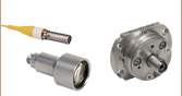
| Fixed FC, APC, or SMA Fiber Collimators | 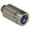 |
These fiber collimation packages are pre-aligned to collimate light from an FC/PC-, FC/APC-, or SMA-terminated fiber. Each collimation package is factory aligned to provide diffraction-limited performance for wavelengths ranging from 405 nm to 4.55 µm. Although it is possible to use the collimator at detuned wavelengths, they will only perform optimally at the design wavelength due to chromatic aberration, which causes the effective focal length of the aspheric lens to have a wavelength dependence. |
| Air-Spaced Doublet, Large Beam Collimators | 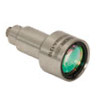 |
For large beam diameters (Ø5.3 - Ø8.5 mm), Thorlabs offers FC/APC, FC/PC, and SMA air-spaced doublet collimators. These collimation packages are pre-aligned at the factory to collimate a laser beam propagating from the tip of an FC or SMA-terminated fiber and provide diffraction-limited performance at the design wavelength. |
| Triplet Collimators | 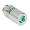 |
Thorlabs' High Quality Triplet Fiber Collimation packages use air-spaced triplet lenses that offer superior beam quality performance when compared to aspheric lens collimators. The benefits of the low-aberration triplet design include an M2 term closer to 1 (Gaussian), less divergence, and less wavefront error. |
| Achromatic Collimators for Multimode Fiber | 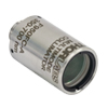 |
Thorlabs' High-NA Achromatic Collimators pair a meniscus lens with an achromatic doublet for high performance across the visible spectrum with low spherical aberration. Designed for use with high-NA multimode fiber, these collimators are ideal for Optogenetics and Fiber Photometry applications. |
| Reflective Collimators | 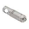 |
Thorlabs' metallic-coated Reflective Collimators are based on a 90° off-axis parabolic mirror. Mirrors, unlike lenses, have a focal length that remains constant over a broad wavelength range. Due to this intrinsic property, a parabolic mirror collimator does not need to be adjusted to accommodate various wavelengths of light, making them ideal for use with polychromatic light. Our reflective collimators are ideal for collimating single mode fiber but are not recommended for coupling into single mode fiber. We also offer a compact version of the protected-silver-coated reflective collimators that is directly compatible with our 16 mm cage system. |
| FiberPorts | 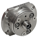 |
These compact, ultra-stable FiberPort micropositioners provide an easy-to-use, stable platform for coupling light into and out of FC/PC, FC/APC, or SMA terminated optical fibers. It can be used with single mode, multimode, or PM fibers and can be mounted onto a post, stage, platform, or laser. The built-in aspheric or achromatic lens is available with five different AR coatings and has five degrees of alignment adjustment (3 translational and 2 pitch). The compact size and long-term alignment stability make the FiberPort an ideal solution for fiber coupling, collimation, or incorporation into OEM systems. |
| Adjustable Fiber Collimators |  |
These collimators are designed to connect onto the end of an FC/PC, FC/APC, or SMA connector and contain an AR-coated aspheric lens. The distance between the aspheric lens and the tip of the fiber can be adjusted to compensate for focal length changes or to recollimate the beam at the wavelength and distance of interest. |
| Achromatic Fiber Collimators with Adjustable Focus | 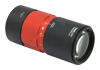 |
Thorlabs' Achromatic Fiber Collimators with Adjustable Focus are designed with an effective focal length (EFL) of 20 mm, 40 mm, or 80 mm, have optical elements broadband AR coated for one of three wavelength ranges, and are available with FC/PC, FC/APC, or SMA905 connectors. A four-element, air-spaced lens design produces superior beam quality (M2 close to 1) and less wavefront error when compared to aspheric lens collimators. These collimators can be used for free-space coupling into a fiber, collimation of output from a fiber, or in pairs for collimator-to-collimator coupling over long distances, which allows the beam to be manipulated prior to entering the second collimator. |
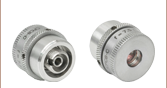
| Zoom Fiber Collimators | 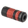 |
These collimators provide a variable focal length between 6 and 18 mm, while maintaining the collimation of the beam. As a result, the size of the beam can be changed without altering the collimation. This universal device saves time previously spent searching for the best suited fixed fiber collimator and has a very broad range of applications. They are offered with FC/PC, FC/APC, or SMA905 connectors with three different antireflection wavelength ranges to choose from. |
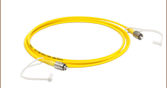
| Single Mode Pigtailed Collimators | 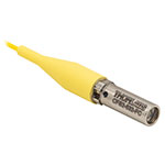 |
Our single mode pigtailed collimators come with one meter of fiber, consist of an AR-coated aspheric lens pre-aligned with respect to a fiber, and are collimated at one of eight wavelengths: 532 nm, 633 nm, 780 nm, 850 nm, 1030 nm, 1064 nm, 1310 nm, or 1550 nm. Although it is possible to use the collimator at any wavelength within the coating range, the coupling loss will increase as the wavelength is detuned from the design wavelength. |
| Polarization Maintaining Pigtailed Collimators | 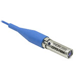 |
Our polarization maintaining pigtailed collimators come with one meter of fiber, consist of an AR-coated aspheric lens pre-aligned with respect to a fiber, and are collimated at one of six wavelengths: 532 nm, 830 nm, 1030 nm, 1064 nm, 1310 nm, or 1550 nm. Custom wavelengths and connectors are available as well. A line is engraved along the outside of the housing that is parallel to the slow axis. As such, it can be used as a reference when polarized light is launched accordingly. Although it is possible to use the collimator at any wavelength within the coating range, the coupling loss will increase as the wavelength is detuned from the design wavelength. |
| GRIN Fiber Collimators |  |
Thorlabs offers gradient index (GRIN) fiber collimators that are aligned at a variety of wavelengths from 630 to 1550 nm and have either FC terminated, APC terminated, or unterminated fibers. Our GRIN collimators feature a Ø1.8 mm clear aperture, are AR-coated to ensure low back reflection into the fiber, and are coupled to standard single mode or graded-index multimode fibers. |
| GRIN Lenses |  |
These graded-index (GRIN) lenses are AR coated for applications at 630, 830, 1060, 1300, or 1560 nm that require light to propagate through one fiber, then through a free-space optical system, and finally back into another fiber. They are also useful for coupling light from laser diodes into fibers, coupling the output of a fiber into a detector, or collimating laser light. Our GRIN lenses are designed to be used with our Pigtailed Glass Ferrules and GRIN/Ferrule sleeves. |

 Zoom
ZoomThorlabs' FC/PC-Terminated Zoom Fiber Collimators provide a variable focal length (6 mm to 18 mm) and feature an FC/PC 2.2 mm wide key connector. They are AR-coated for three different wavelength ranges (400 nm - 650 nm, 650 nm - 1050 nm, or 1050 nm - 1650 nm). In order to take full advantage of the superior beam quality, we recommend using our zoom collimators with our AR-coated single mode or polarization-maintaining fiber optic patch cables. These cables, which are available with an FC/PC 2.0 mm narrow key connector, have an antireflective coating on one fiber end for increased transmission and improved return loss at the fiber-to-free-space interface.
These zoom collimator packages use high-precision 2.2 mm wide key connectors with tightly toleranced ceramic sleeves that provide excellent pointing repeatability, allowing the user to easily remove and replace the fiber. Please note that careful alignment is needed when mating a narrow key PM fiber with the collimator's wide key receptacle.
When using one of these collimators as a free-space coupler, precise alignment is needed for good coupling efficiency. We recommend using a kinematic tip and tilt mount paired with an XYZ adjustable platform, such as our KM100T and MT3(MT3/M) or our K6XS 6-axis kinematic mount. Additionally, the zoom collimators may be used in pairs with a free-space beam in between. This free-space beam can be manipulated with many types of optics prior to entering the second collimator.
Performance of each collimator can be obtained by the using the black box Zemax files (See the Zemax Files tab for more information).

 Zoom
ZoomThorlabs' FC/APC-Terminated Zoom Fiber Collimators provide a variable focal length (6 mm to 18 mm) and feature an FC/APC 2.2 mm wide key connector. They are AR-coated for three different wavelength ranges (400 nm - 650 nm, 650 nm - 1050 nm, or 1050 nm - 1650 nm). In order to take full advantage of the superior beam quality, we recommend using our zoom collimators with our AR-coated single mode or polarization-maintaining fiber optic patch cables. These cables, which are available with an FC/APC 2.0 mm narrow key connector, have an antireflective coating on one fiber end for increased transmission and improved return loss at the fiber-to-free-space interface.
These zoom collimator packages use high-precision 2.2 mm wide key connectors with tightly toleranced ceramic sleeves that provide excellent pointing repeatability, allowing the user to easily remove and replace the fiber. Please note that careful alignment is needed when mating a narrow key PM fiber with the collimator's wide key receptacle. The receptacles for the APC connectors are angled so that light exiting the fiber enters the collimator perpendicular to the focal plane.
When using one of these collimators as a free-space coupler, precise alignment is needed for good coupling efficiency. We recommend using a kinematic tip and tilt mount paired with an XYZ adjustable platform, such as our KM100T and MT3(MT3/M) or our K6XS 6-axis kinematic mount. Additionally, the zoom collimators may be used in pairs with a free-space beam in between. This free-space beam can be manipulated with many types of optics prior to entering the second collimator.
Performance of each collimator can be obtained by the using the black box Zemax files (See the Zemax Files tab for more information).

 Zoom
ZoomThorlabs' SMA-Terminated Zoom Fiber Collimators provide a variable focal length (6 mm to 18 mm) and feature an SMA905 connector. They are AR-coated for three different wavelength ranges (400 nm - 650 nm, 650 nm - 1050 nm, or 1050 nm - 1650 nm). These collimators are designed for applications that require multimode fibers; we recommend using the AR-coated multimode fiber optic patch cables (see the Multimode tab for details).
When using one of these collimators as a free-space coupler, precise alignment is needed for good coupling efficiency. We recommend using a kinematic tip and tilt mount paired with an XYZ adjustable platform, such as our KM100T and MT3(MT3/M) or our K6XS 6-axis kinematic mount. Additionally, the zoom collimators may be used in pairs with a free-space beam in between. This free-space beam can be manipulated with many types of optics prior to entering the second collimator.
Performance of each collimator can be obtained by the using the black box Zemax files (See the Zemax Files tab for more information).