 Products Home
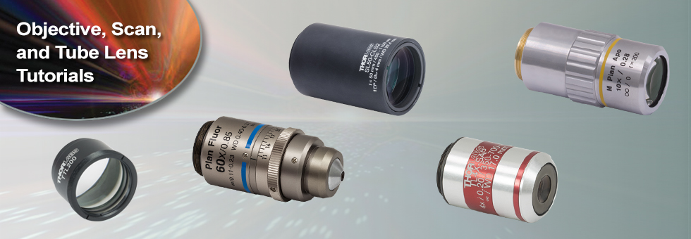
Microscope Objective, Tube, and Scan Lens Tutorials

Please Wait
The tutorials on this page discuss topics related to the function, specification, and operation of objective lenses within an optical system. To navigate to these tutorials, use the Table of Contents below or click on the tabs above.
Table of Contents

Objective Identification
Note: While the diagrams above show typical markings, they serve only as examples. The format and content of the engraved specifications will vary between objectives and manufacturers.
| Magnification Color Codes |
|---|
| Immersion Media Color Codes |
|---|
Types of Objectives
Thorlabs offers several types of objectives to meet a variety of experimental needs. This guide describes the features and benefits of each type of objective.
Dry, Immersion, and Dipping Objectives
This designation refers to the medium that should be present between the front of the objective and the cover glass of the microscope slide. Dry objectives are designed to work best with an air gap between the objective and the specimen. Oil-immersion objectives require the use of a drop of immersion oil (such as MOIL-30) between and in contact with the front lens of the objective and the cover glass. Oil immersion is required in order to achieve numerical apertures greater than 1.0. Water-immersion (coverslip) objectives are designed to work best with a drop of water between the objective and specimen, while water-dipping objectives are designed to interface directly with the specimen. Note that if an immersion or dipping objective is used without the immersion medium present, the image quality will be very low.
Plan Achromat and Plan Apochromat Objectives
"Plan" designates that these objectives produce a flat image across the field of view. "Achromat" refers to the correction for chromatic aberration featured in the lens design. These objectives have chromatic aberration correction for two wavelengths and spherical aberration correction at one wavelength. Plan achromats produce their best images for green light. Apochromat objectives have chromatic aberration correction for three to five wavelengths and spherical aberration correction at two to four wavelengths. In white light, the plan achromats give satisfactory images for color photomicrography, but the results are not as good as objectives that feature better correction, such as plan apochromats or the plan fluorite objectives below.
Plan Fluorite Objectives
Plan fluorite objectives, also referred to as plan semi-apochromats, plan fluorescence objectives, or plan fluors, also produce a flat image across the field of view. Plan fluorite objectives are corrected for chromatic aberrations at two to four wavelengths and spherical aberrations at three to four wavelengths. In addition to being corrected for more wavelengths, plan fluorite objectives generally offer reduced aberrations between the design wavelengths relative to plan achromats. These objectives also work well for color photomicrography.
Super Apochromat Objectives
Thorlabs' super apochromat objectives feature axial color correction throughout the visible range. They are designed to provide diffraction-limited axial color performance over a wide field of view with no vignetting over the entire field. The high NA of the super apochromatic design makes them ideal for widefield imaging and light-starved environments.
Glossary of Terms
Magnification
The magnification of an objective is the lens tube focal length (L) divided by the objective's focal length (F):
M = L / F .
The total magnification of the system is the magnification of the objective multiplied by the magnification of the eyepiece or camera tube. The specified magnification on the microscope objective housing is accurate as long as the objective is used with a compatible tube lens focal length.
Numerical Aperture (NA)
Numerical aperture, a measure of the acceptance angle of an objective, is a dimensionless quantity. It is commonly expressed as
NA = ni × sinθa
where θa is the maximum 1/2 acceptance angle of the objective, and ni is the index of refraction of the immersion medium. This medium is typically air, but may also be water, oil, or other substances.
Parfocal Length
Also referred to as the parfocal distance, this is the length from the top of the objective (at the base of the mounting thread) to the bottom of the cover glass (or top of the specimen in the case of objectives that are intended to be used without a cover glass). Parfocal length is not the same from manufacturer to manufacturer or even within the same manufacturer. For instance, Thorlabs manufactures objectives with 60 mm and 95 mm parfocal lengths, many Olympus and Zeiss objectives have a parfocal length of 45 mm, and the standard for Nikon and Leica objectives is 60 mm. Furthermore, some manufacturers also offer oversized objectives with a 75 mm parfocal length. For instances in which objectives with different parfocal lengths must be used, parfocal length extenders are available.
Working Distance
This is the distance between the front element of the objective and the closest surface of the coverslip or specimen, depending on the design of the objective. The cover glass thickness specification engraved on the objective designates whether a cover glass should be used.
Click to Enlarge
This graph shows the effect of a cover slip on image quality at 632.8 nm.
Field Number
The field number corresponds to the size of the field of view (in millimeters) multiplied by the objective's magnification.
FN = Field of View Diameter × Magnification
Coverslip Correction and Correction Collar (Ring)
A typical coverslip (cover glass) is designed to be 0.17 mm thick, but due to variance in the manufacturing process the actual thickness may be different. The correction collar present on select objectives is used to compensate for coverslips of different thickness by adjusting the relative position of internal optical elements. Note that many objectives do not have a variable coverslip correction (for example, an objective could be designed for use with only a standard 0.17 mm thick coverglass), in which case the objectives have no correction collar.
The graph to the right shows the magnitude of spherical aberration versus the thickness of the coverslip used, for 632.8 nm light. For the typical coverslip thickness of 0.17 mm, the spherical aberration caused by the coverslip does not exceed the diffraction-limited aberration for objectives with NA up to 0.40.
When viewing an image with a camera, the system magnification is the product of the objective and camera tube magnifications. When viewing an image with trinoculars, the system magnification is the product of the objective and eyepiece magnifications.

| Manufacturer | Tube Lens Focal Length |
|---|---|
| Leica | f = 200 mm |
| Mitutoyo | f = 200 mm |
| Nikon | f = 200 mm |
| Olympus | f = 180 mm |
| Thorlabs | f = 200 mm |
| Zeiss | f = 165 mm |
Magnification and Sample Area Calculations
Magnification
The magnification of a system is the multiplicative product of the magnification of each optical element in the system. Optical elements that produce magnification include objectives, camera tubes, and trinocular eyepieces, as shown in the drawing to the right. It is important to note that the magnification quoted in these products' specifications is usually only valid when all optical elements are made by the same manufacturer. If this is not the case, then the magnification of the system can still be calculated, but an effective objective magnification should be calculated first, as described below.
To adapt the examples shown here to your own microscope, please use our Magnification and FOV Calculator, which is available for download by clicking on the red button above. Note the calculator is an Excel spreadsheet that uses macros. In order to use the calculator, macros must be enabled. To enable macros, click the "Enable Content" button in the yellow message bar upon opening the file.
Example 1: Camera Magnification
When imaging a sample with a camera, the image is magnified by the objective and the camera tube. If using a 20X Nikon objective and a 0.75X Nikon camera tube, then the image at the camera has 20X × 0.75X = 15X magnification.
Example 2: Trinocular Magnification
When imaging a sample through trinoculars, the image is magnified by the objective and the eyepieces in the trinoculars. If using a 20X Nikon objective and Nikon trinoculars with 10X eyepieces, then the image at the eyepieces has 20X × 10X = 200X magnification. Note that the image at the eyepieces does not pass through the camera tube, as shown by the drawing to the right.
Using an Objective with a Microscope from a Different Manufacturer
Magnification is not a fundamental value: it is a derived value, calculated by assuming a specific tube lens focal length. Each microscope manufacturer has adopted a different focal length for their tube lens, as shown by the table to the right. Hence, when combining optical elements from different manufacturers, it is necessary to calculate an effective magnification for the objective, which is then used to calculate the magnification of the system.
The effective magnification of an objective is given by Equation 1:
 |
(Eq. 1) |
Here, the Design Magnification is the magnification printed on the objective, fTube Lens in Microscope is the focal length of the tube lens in the microscope you are using, and fDesign Tube Lens of Objective is the tube lens focal length that the objective manufacturer used to calculate the Design Magnification. These focal lengths are given by the table to the right.
Note that Leica, Mitutoyo, Nikon, and Thorlabs use the same tube lens focal length; if combining elements from any of these manufacturers, no conversion is needed. Once the effective objective magnification is calculated, the magnification of the system can be calculated as before.
Example 3: Trinocular Magnification (Different Manufacturers)
When imaging a sample through trinoculars, the image is magnified by the objective and the eyepieces in the trinoculars. This example will use a 20X Olympus objective and Nikon trinoculars with 10X eyepieces.
Following Equation 1 and the table to the right, we calculate the effective magnification of an Olympus objective in a Nikon microscope:
 |
The effective magnification of the Olympus objective is 22.2X and the trinoculars have 10X eyepieces, so the image at the eyepieces has 22.2X × 10X = 222X magnification.
Sample Area When Imaged on a Camera
When imaging a sample with a camera, the dimensions of the sample area are determined by the dimensions of the camera sensor and the system magnification, as shown by Equation 2.
 |
(Eq. 2) |
The camera sensor dimensions can be obtained from the manufacturer, while the system magnification is the multiplicative product of the objective magnification and the camera tube magnification (see Example 1). If needed, the objective magnification can be adjusted as shown in Example 3.
As the magnification increases, the resolution improves, but the field of view also decreases. The dependence of the field of view on magnification is shown in the schematic to the right.
Example 4: Sample Area
The dimensions of the camera sensor in Thorlabs' previous-generation 1501M-USB Scientific Camera are 8.98 mm × 6.71 mm. If this camera is used with the Nikon objective and trinoculars from Example 1, which have a system magnification of 15X, then the image area is:
 |
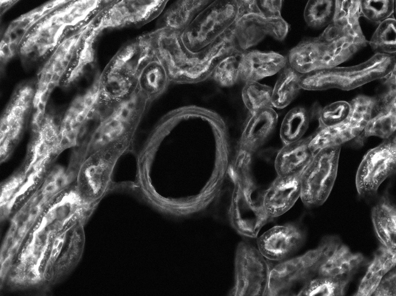
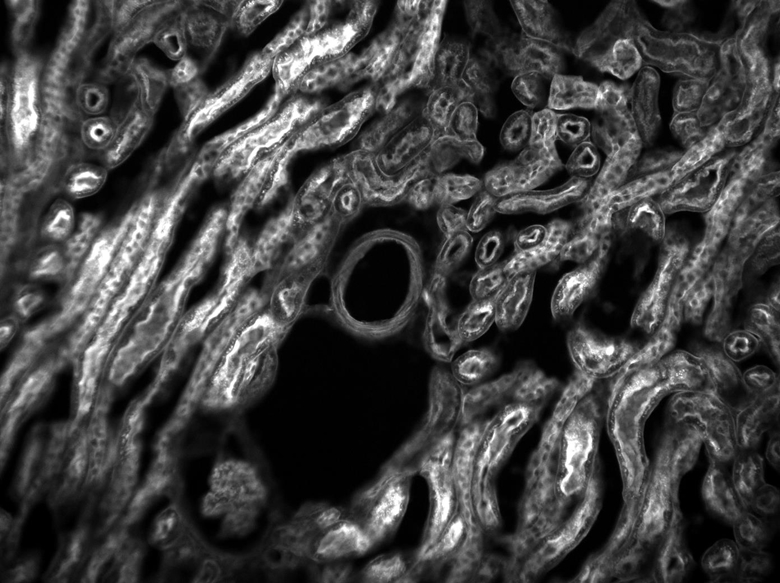
Sample Area Examples
The images of a mouse kidney below were all acquired using the same objective and the same camera. However, the camera tubes used were different. Read from left to right, they demonstrate that decreasing the camera tube magnification enlarges the field of view at the expense of the size of the details in the image.

Resolution Tutorial
An important parameter in many imaging applications is the resolution of the objective. This tutorial describes the different conventions used to define an objective's resolution. Thorlabs provides the theoretical Rayleigh resolution for all of the imaging objectives offered on our site; the other conventions are presented for informational purposes.
Resolution
The resolution of an objective refers to its ability to distinguish closely-spaced features of an object. This is often theoretically quantified by considering an object that consists of two point sources and asking at what minimum separation can these two point sources be resolved. When a point source is imaged, rather than appearing as a singular bright point, it will appear as a broadened intensity profile due to the effects of diffraction. This profile, known as an Airy disk, consists of an intense central peak with surrounding rings of much lesser intensity. The image produced by two point sources in proximity to one another will therefore consist of two overlapping Airy disk profiles, and the resolution of the objective is therefore determined by the minimum spacing at which the two profiles can be uniquely identified. There is no fundamental criterion for establishing what exactly it means for the two profiles to be resolved and, as such, there are a few criteria that are observed in practice. In microscopic imaging applications, the two most commonly used criteria are the Rayleigh and Abbe criteria. A third criterion, more common in astronomical applications, is the Sparrow criterion.
Rayleigh Criterion
The Rayleigh criterion states that two overlapping Airy disk profiles are resolved when the first intensity minimum of one profile coincides with the intensity maximum of the other profile [1]. It can be shown that the first intensity minimum occurs at a radius of 1.22λf/D from the central maximum, where λ is the wavelength of the light, f is the focal length of the objective, and D is the entrance pupil diameter. Thus, in terms of the numerical aperture (NA = 0.5*D/f), the Rayleigh resolution is:
rR = 0.61λ/NA
An idealized image of two Airy disks separated by a distance equal to the Rayleigh resolution is shown in the figure to the left below; the illumination source has been assumed to be incoherent. A corresponding horizontal line cut across the intensity maxima is plotted to the right. The vertical dashed lines in the intensity profile show that the maximum of each individual Airy disk overlaps with the neighboring minimum. Between the two maxima, there is a local minimum which appears in the image as a gray region between the two white peaks.
 Click to Enlarge
Left: Two point sources are considered resolved when separated by the Rayleigh resolution. The gray region between the two white peaks is clearly visible.
Above: The vertical dashed lines show how the maximum of each intensity profile overlaps with the first minimum of the other.

Thorlabs provides the theoretical Rayleigh resolution for all of the imaging objectives offered on our site in their individual product presentations.
Abbe Criterion
The Abbe theory describes image formation as a double process of diffraction [2]. Within this framework, if two features separated by a distance d are to be resolved, at a minimum both the zeroth and first orders of diffraction must be able to pass through the objective's aperture. Since the first order of diffraction appears at the angle: sin(θ1) = λ/d, the minimum object separation, or equivalently the resolution of the objective, is given by d = λ/n*sin(α), where α is the angular semi-aperture of the objective and a factor of n has been inserted to account for the refractive index of the imaging medium. This result overestimates the actual limit by a factor of 2 because both first orders of diffraction are assumed to be accepted by the objective, when in fact only one of the first orders must pass through along with the zeroth order. Dividing the above result by a factor of 2 and using the definition of the numerical aperture (NA = n*sin(α)) gives the famous Abbe resolution limit:
rA = 0.5λ/NA
In the image below, two Airy disks are shown separated by the Abbe resolution limit. Compared to the Rayleigh limit, the decrease in intensity at the origin is much harder to discern. The horizontal line cut to the right shows that the intensity decreases by only ≈2%.
 Click to Enlarge
Left: Two point sources separated by the Abbe resolution limit. Though observable, the contrast between the maxima and central minimum is much weaker compared to the Rayleigh limit.
Above: The line cut shows the small intensity dip between the two maxima.

Sparrow Criterion
For point source separations corresponding to the Rayleigh and Abbe resolution criteria, the combined intensity profile has a local minimum located at the origin between the two maxima. In a sense, this feature is what allows the two point sources to be resolved. That is to say, if the sources' separation is further decreased beyond the Abbe resolution limit, the two individual maxima will merge into one central maximum and resolving the two individual contributions will no longer be possible. The Sparrow criterion posits that the resolution limit is reached when the crossover from a central minimum to a central maximum occurs.
At the Sparrow resolution limit, the center of the combined intensity profile is flat, which implies that the derivative with respect to position is zero at the origin. However, this first derivative at the origin is always zero, given that it is either a local minimum or maximum of the combined intensity profile (strictly speaking, this is only the case if the sources have equal intensities). Consider then, that because the Sparrow resolution limit occurs when the origin's intensity changes from a local minimum to a maximum, that the second derivative must be changing sign from positive to negative. The Sparrow criterion is thus a condition that is imposed upon the second derivative, namely that the resolution limit occurs when the second derivative is zero [3]. Applying this condition to the combined intensity profile of two Airy disks leads to the Sparrow resolution:
rS = 0.47λ/NA
The image to the left below shows two Airy disks separated by the Sparrow resolution limit. As described above, the intensity is constant in the region between the two peaks and there is no intensity dip at the origin. In the line cut to the right, the constant intensity near the origin is confirmed.
 Click to Enlarge
Left: Two Airy disk profiles separated by the Sparrow resolution limit. Note that, unlike the Rayleigh or Abbe limits, there is no decrease in intensity at the origin.
Above: At the Sparrow resolution limit, the combined intensity is a constant near the origin. The scale here has been normalized to 1.

References
[1] Eugene Hecht, "Optics," 4th Ed., Addison-Wesley (2002)
[2] S.G. Lipson, H. Lipson, and D.S. Tannhauser, "Optical Physics," 3rd Ed., Cambridge University Press (1995)
[3] C.M. Sparrow, "On Spectroscopic Resolving Power," Astrophys. J. 44, 76-87 (1916)
 Click to Enlarge
Figure 1: A Gaussian intensity profile only asymptotically approaches zero, so the spot size is defined by convention as either the full-width at half-maximum (FWHM) or 1/e2 value. We use the latter convention in this tutorial.
Spot Size Tutorial
The spot size achieved by focusing a laser beam with a lens or objective is an important parameter in many applications. This tutorial describes how the ratio of the initial beam diameter to the entrance pupil diameter, known as the truncation ratio, affects the focused spot size and provides expressions for calculating the spot size as a function of this ratio. Because the power transmitted by the focusing optic also depends upon the truncation ratio, the optimal balance between spot size and power transmission will depend upon the given application.
For each focusing objective that Thorlabs provides, we provide an estimate of the focused spot size when the incident Gaussian spot size (1/e2) is the same as the diameter of the entrance pupil. With this choice, the focused spot size is given by:
s ≈ 1.83λN, or equivalently, s ≈ 1.83λ/(2*NA), where NA is the numerical aperture of the objective; and the transmitted power is 86% of that of the incident beam.
Gaussian Beam Profile
Laser beams typically have a tranverse intensity profile that may be approximated by a Gaussian function,![]() ,
,
where w is the beam half-width or beam waist radius, conventionally defined as the radius (r) at which the intensity has decreased from its maximum axial value of I0 to I0/e2 ≈ 0.14I0. The spot size of a laser beam may be defined as twice the beam waist radius, and the corresponding circle with diameter equal to the spot size thus contains 86% of the beam's total intensity.
When a laser beam is focused by an objective, the resulting spot size (s) will depend upon the wavelength of the light (λ), the beam diameter as it enters the objective (S), the focal length of the objective (f), and the entrance pupil diameter of the objective (D). Dimensionless parameters are formed by taking the ratio of the focal length to the entrance pupil diameter and the ratio of the beam diameter to the entrance pupil diameter, which are known respectively as the f-number (N = f/D) and the truncation ratio (T = S/D). The f-number is fixed for a given objective, while the truncation ratio may be tuned by increasing or decreasing the incident beam diameter.
Spot Size vs. Truncation Ratio
The focused spot size is expressed in terms of the wavelength, truncation ratio, and f-number as
![]()
where K(T) is called the spot size coefficient and is a function of the truncation ratio [1]. In Figure 2 below, numerically computed values for K, obtained by calculating the focused intensity profile and extracting the focused spot size for discrete values of T, are plotted as black squares. As discussed in detail below, the solid-and-dashed blue line represents the coefficient predicted by Gaussian beam theory, the gray line represents the value of K for an Airy disk intensity profile, and the red line is a polynomial fit to the numerical values for T ≥ 0.5.
 Click to Enlarge
Figure 2: The shaded blue region below T < 0.5 indicates where Gaussian beam theory provides an accurate estimate of the focused spot size; however, above this value the effects of truncation cannot be neglected and the actual spot size is larger. As T → ∞, the coefficient approaches the Airy disk value of 1.6449 as indicated by the solid gray line.
 Click to Enlarge
Figure 3: The power transmitted through an entrance aperture of diameter D by a Gaussian beam with spot size S as a function of the truncation ratio T = S/D. The shaded blue region corresponds to the region where truncation effects on the spot size are negligible.
In both the large (T → ∞) and small (T → 0) limits, K approaches well-known theoretical results. For small T, which corresponds to an entrance pupil much larger than the Gaussian spot, K obeys the relation 1.27/T. This can be obtained from Gaussian beam propagation theory [2] which predicts that the minimum spot size a Gaussian beam can be focused to is s ≈ 1.27λf/S. By inserting factors of D to write this in terms of N and T, this expression can be cast into the same form as the spot size equation above, s = (1.27/T)λN, giving the result K = 1.27/T. As seen in Figure 2 above, this accurately predicts the focused spot size up to T ≈ 0.5, when the entrance pupil diameter D is twice as large as the spot size S. Above T = 0.5, it underestimates the value of K, as indicated by the deviation of the dashed blue line from the numerical results.
 Click to Enlarge
Figure 4: The spot size of an Airy disk profile is typically defined by the radius where the first intensity zero occurs. When the radius is expressed in units of λN, this corresponds to a radius of 1.22λN, or a spot size of 2.44λN. The 1/e2 radius for the same profile is 0.82245λN, or a spot size of 1.6449λN.
As T is increased, the illumination of the aperture becomes more and more uniform. The resulting intensity profile of the focused spot will therefore transition from a Gaussian profile to an Airy disk profile. In the large T limit, this is reflected in the value of K, which approaches a constant value of 1.6449 as T → ∞. This value corresponds to the 1/e2 spot size of an Airy disk instead of the better-known 2.44λN value which is where the first intensity minimum occurs, as shown in Figure 4 [3].
For intermediate values of T, which is the range in which most applications will fall, there is no exact theoretical result for K. Instead, the red line above represents a two-term polynomial fit to the numerical results, the coefficients of which are specified in the table below (the polynomial fit was performed using 1/T as the independent variable). This expression may be used to estimate K for T ≥ 0.5.
| Spot Size Coefficient, K(T) | |
|---|---|
| Truncation Ratio | Equation |
| T < 0.5 (Gaussian Regime) |
|
| T ≥ 0.5 (Intermediate and Uniform/Airy Regimes) |
|
Power Transmission and Spot Size
The results presented above suggest that, in the intermediate T regime, a smaller spot size may be achieved by increasing T. This, however, comes at the cost of reducing the overall power transmitted through the entrance aperture, and reductions in spot size may not be worth the loss in power. The power transmitted through an entrance pupil of diameter D as a function of T is plotted above in Figure 3. Already at T = 1, when the Gaussian spot size has the same diameter as the entrance pupil, the transmitted power is 86% of the incident power. By increasing T from 1 to 2, the spot size is reduced by only ≈ 9%, while the transmitted power decreases from 86% to 40%.
The optimal balance between spot size and power transmission will depend upon the given application. For each focusing objective that Thorlabs offers, we provide an estimate of the spot size using T = 1, when the Gaussian spot size is the same as the diameter of the entrance pupil. With this choice, the spot size is given by: s ≈ 1.83λN, or equivalently, s ≈ 1.83λ/(2*NA), where NA is the numerical aperture of the objective.
References
[1] Hakan Urey, "Spot size, depth-of-focus, and diffraction ring intensity formulas for truncated Gaussian beams," Appl. Opt. 43, 620-625 (2004)
[2] Sidney A. Self, "Focusing of spherical Gaussian beams," Appl. Opt. 22, 658-661 (1983)
[3] Eugene Hecht, "Optics," 4th Ed., Addison-Wesley (2002)
Scan lenses are used in a variety of laser imaging systems, including confocal laser scanning microscopy, optical coherence tomography (OCT), and multiphoton imaging systems. In these applications, a laser beam incident on the back aperture (entrance pupil) of the lens is scanned through a range of angles. This translates the position of the spot formed in the image plane across the lens' field of view. In the case of non-telecentric lenses, this approach to scanning the focal spot through the image plane would introduce severe aberrations that would significantly degrade the quality of the resulting image. Telecentric scan lenses are designed to create a uniform spot size in the image plane at every scan position, which allows a high-quality image of the sample to be formed.
In general, laser scanning microscopy systems pair a scan lens with a tube lens to create an infinity-corrected optical system. However, most OCT systems are designed to use the scan lens without a tube lens. The CLS-SL, SL50-CLS2, SL50-2P2, and SL50-3P lenses were optimized for use in Thorlabs' confocal laser scanning and multiphoton microscopy systems, and the LSM family of lenses were optimized to be used in OCT imaging systems. A brief discussion of scanning systems implemented with and without tube lenses follows.
Click to Enlarge
The tube and scan lens schematic above shows the lens spacing for the SL50-2P2 scan lens used with a 200 mm focal length telecentric tube lens. Note that for the SL50-CLS2, the entrance pupil at the scan plane is a maximum of Ø4 mm.
Scan Lenses Implemented in General Laser Scanning Microscopy Applications
The image to the right shows the proper spacing of the scan and tube lenses for laser scanning microscopy. The scanning mirror, which is located at the left of the image at the scan plane, directs the laser beam through the scan lens. The angle at which the laser beam is incident on the scan lens determines the position of the focal spot in the intermediate image plane, which is located between the scan lens and the ITL200 tube lens. The tube lens is positioned so that it collects and collimates the light (the focus is at infinity). The collimated light is collected by the objective, which brings it to a focus on the sample plane. Light scattered or emitted from the sample plane is collected by the objective and directed to a detector. The image below and to the left shows a CLS-SL scan lens paired with a tube lens; clicking on the image shows the correct spacing for using the CLS-SL with the ITL200 tube lens.
An attractive feature of this optical system design is the collimated light that is produced as a result of pairing the scan lens with the tube lens. With the light from the tube lens focusing at infinity, it is possible to move the position of the objective with respect to the tube lens without impacting the image quality at the sample plane. This imparts considerable flexibility to the design of the optical system. If no tube lens were used, the scan lens would also function as the objective and the intermediate image plane would become the sample plane. It would not be possible to move the image plane much with respect to the scan lens while maintaining image quality.
The image below and to the right shows the relationship between the scan distance and the objective distance. In a perfect 4f optical system (using the CLS-SL as an example), d1 = 52 mm (minimum scan distance) and d2 = f2. However, in many practical cases the system is slightly deviated from this perfect alignment. For instance, in many commercial microscopes, the objective distance (d2) is not the same as the focal length (f2), so there may be a need to adjust distances. The figure below and to the right shows the scan and objective distance moved by some small distance δ1 and δ2, respectively. The relationship between these values is δd1 = -δd2*(f1/f2)2.
Click for Details
CLS-SL Tube Lens integration with the ITL200 and an objective in a laser scanning system.
Click to Enlarge
A diagram showing lens placement for a general laser scanning system.
Scan Lenses Implemented in OCT
When designing an imaging system that uses an LSM scan lens in an OCT configuration, it is important to accommodate the design wavelength, parfocal distance, scanning distance, entrance pupil, and scan angle specifications in order to maximize the image quality. In general, the larger the input beam diameter, the smaller the focused spot size. However, due to the effects of vignetting and/or increased aberrations, the range of scan angles decreases as the diameter of the beam increases. Beams smaller than the entrance pupil specification will result in spot sizes larger than those specified for the scan lens, and beams with larger diameters will be clipped.
For imaging systems with a single galvo mirror the center of the scan lens' entrance pupil is coincident with the pivot point of the galvo mirror. When a single galvo mirror is used, the scanning distance is measured from the mounting surface of the lens to the pivot point of the mirror. This is shown in the image at bottom-left.
If the imaging system uses two galvo mirrors (one to scan in the X direction and one to scan in the Y direction), the entrance pupil is located between the two galvo mirrors, as is shown in the image at bottom-right. The scanning distance is then the distance from the mounting surface of the lens to the pivot point of the mirror closest to the lens (d1) plus the distance from the pivot point of that mirror to the entrance pupil (d2). It is important to minimize the distance between the two galvo mirrors, because when the entrance pupil and beam steering pivot point are not coincident, the quality of the image is degraded. This is principally due to the variation in the optical path length as the beam is scanned over the sample. Below are schematics for an imaging system containing one and two galvo mirrors.
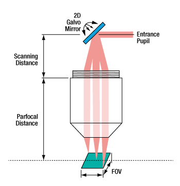
When one galvo mirror is used, the entrance pupil is located
at the pivot point of the mirror.
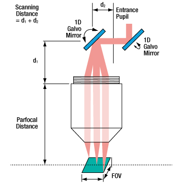
When two galvo mirrors are used, the entrance pupil is located between the mirrors.
| Posted Comments: | |
user
(posted 2021-07-10 05:46:52.447) I am building my own tube lens. It seems to focus fine, however, I can only detect the signal from the sample on the glass but not under a coverslip. Is there any explanation why? There is still room to put the sample located under the coverslip in the lens tube focal point. YLohia
(posted 2021-07-15 11:03:53.0) Hello, it appears that your system is not well aligned and the sample is not in focus. Another possibility is that your coverslip surface has some defects and is scattering your signal. Qiaoqiao Xue
(posted 2019-09-26 19:42:26.333) Unable to open scanning lens LSM02, thread too tight YLohia
(posted 2019-10-14 09:09:57.0) Hello, thank you for contacting Thorlabs. We have reached out to you directly to gather more information to troubleshoot your issue. |