 Products Home / Optomechanical Components / Optomechanical Mounts / Rotation Mounts / Compact Direct Drive Rotation Mount
Compact Direct Drive Rotation Mount

- Rotational Speeds Up to 5.0 Hz
- SM05 (0.535"-40) Threaded Central Bore
- 16 mm and 30 mm Cage System Compatible
- Backlash-Free Direct-Drive Design
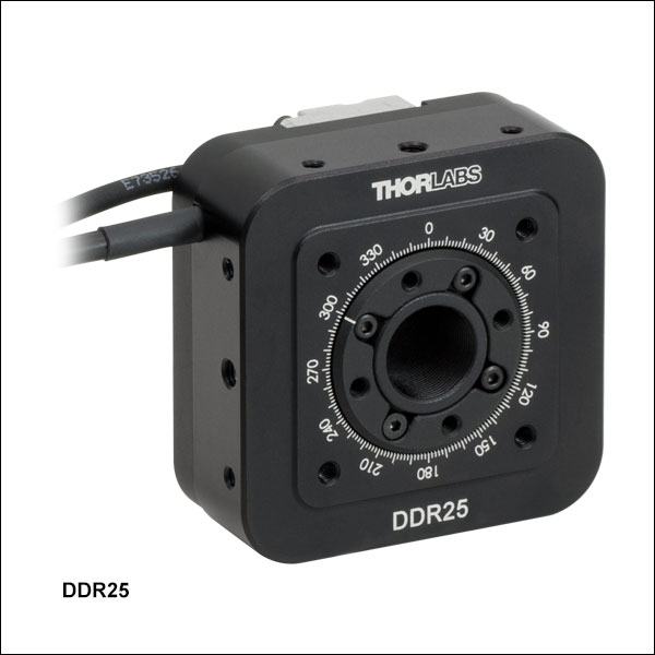
DDR25
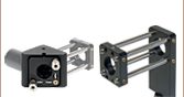
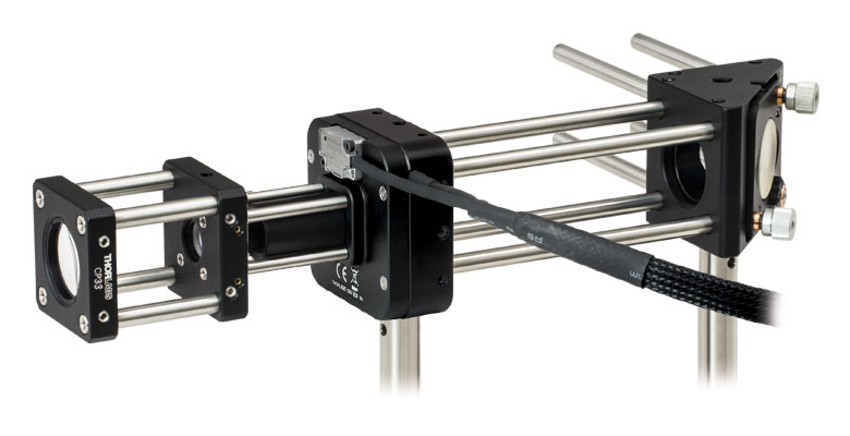
Application Idea
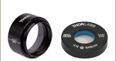
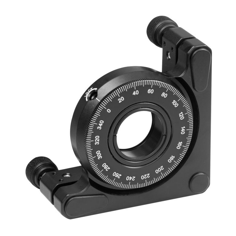
Ø1" Linear Film Polarizer in a CRM1T Rotation Mount and Ø1/2" Linear Film Polarizer Threaded into the DDR25 Motorized Rotation Mount


Please Wait
| Key Specificationsa | |
|---|---|
| Travel Range | 360° Continuous |
| Maximum Velocity | 5.0 Hz (1800 °/s) |
| Maximum Acceleration | 29.1 Hz/s (10477 °/s2) |
| Bidirectional Repeatability | 60 µrad (0.00344°) |
| Maximum Moment of Inertia of Load About Rotation Axis |
70 kg•mm2 |
| Central Aperture | SM05 (0.535"-40) Threaded Bore |
| Motor Type | Brushless DC Rotary Motor |
| Cable Length | 3.0 m (9.8') |
| Required Controller (Sold Separately) | KBD101 |
| Mount Dimensions (L x W x H) | 55.6 mm x 55.6 mm x 28.5 mm (2.19" x 2.19" x 1.12") |
Click to Enlarge
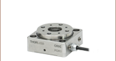
The rear face of the rotation stage (shown) has four stationary tapped holes for 16 mm cage system rods. A 30 mm cage system can be continued from the back side of the stage by using an SP15(/M) 30 mm to 16 mm Cage Adapter Plate.
Features
- 360° Continuous Rotation
- High Speeds up to 5.0 Hz (1800 °/s)
- SM05 (0.535"-40) Threaded Central Bore for Compatibility with Ø1/2" Lens Tubes
- Tapped Holes for 16 mm and 30 mm Cage System Integration
- Compact Design: 55.6 mm x 55.6 mm x 28.5 mm
- Integrated Brushless DC Servo Motor Actuators
- High-Quality, Precision-Engineered Bearings
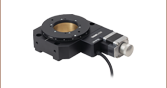
Thorlabs’ DDR25(/M) low-profile, direct-drive rotary mount provides continuous rotation of a load with a moment of inertia up to 70 kg•mm2 with a maximum rotation speed of up to 5.0 Hz (1800 °/s). An SM05 (0.535"-40) threaded central aperture allows an optical path to pass directly through the body of the mount and provides compatibility with Ø1/2" optical elements and Ø1/2" lens tubes. Components can be threaded into this bore from either side of the rotation mount.
The DDR25(/M) has a 3-phase, slotless, brushless DC motor integrated directly into the frame of the stage. This eliminates all forms of mechanical transmission, resulting in high repeatability, rigidity and reliability. The winding design enables good velocity stability, even at low speeds, by eliminating torque ripple due to magnetic cogging. The optical encoder has a 4.3 µrad theoretical resolution and provides high accuracy and repeatability, while the precision-engineered bearings and tight manufacturing tolerances produce low axial wobble. An engraved graduated scale with 2° increments allows for coarse positioning.
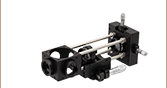
The mount is designed to be mounted vertically on a post using one of four 8-32 (M4) taps on the sides of the device. The rotating portion of the front face features four 4-40 tapped holes spaced for integration of 16 mm cage system assemblies and components, allowing for the rotation of a cage segment. The non-rotating portion of the front face also includes four 4-40 tapped holes spaced for use with 30 mm cage system components. The back of the device features four more 4-40 tapped holes for 16 mm cage system rods, but this portion of the cage remains stationary. A stationary 30 mm cage system can be continued on the back side of the stage using an SP15(/M) 30 mm to 16 mm cage adapter plate, as shown in the image to the right. The position of all of these tapped holes can be seen in the diagram below.
The stage is driven by the KBD101 brushless DC controller (sold separately below), which provides very precise positioning through the stable closed-loop PID control system (see the PID Tutorial tab for more information). The controller ships with our Kinesis and legacy APT software packages for easy integration into an existing system. Power supplies for the K-Cube™ controller are sold separately (see below).
| DDR25(/M) Mount Specifications | |
|---|---|
| Travel Range | 360° Continuous |
| Maximum Velocity | 5.0 Hz (1800 °/s) |
| Maximum Accelerationa | 29.1 Hz/s (10477 °/s2) |
| Bidirectional Repeatability | 60 µrad (0.00344°) |
| Backlashb | None |
| Encoder Resolution | 1.44 x 10⁶ Counts/rev (0.00025 °/Count) |
| Maximum Moment of Inertia of Load About Rotation Axisc |
70 kg•mm2 |
| Minimum Motor Holding Torque | 1.8 N•cm |
| Velocity Stability | ±2.0% (For Speeds 0.5 - 5.0 Hz) |
| Max Wobble (Axial) | 1790 µrad (0.103°) |
| Bearing Type | Deep Groove Ball Bearing |
| Limit Switches | None |
| Central Aperture | SM05 (0.535"-40) Threaded Bore |
| Operating Temperature Ranged | 5 to 40 °C (41 to 104 °F) |
| Motor Type | Brushless DC Rotary Motor |
| Cable Length | 3.0 m (9.8') |
| Required Controller | KBD101 (Sold Separately Below) |
| Stage Dimensions (L x W x H) | 55.6 mm x 55.6 mm x 28.5 mm (2.19" x 2.19" x 1.12") |
| Weight | 0.40 kg (0.88 lbs) |
| KBD101 K-Cube Controller Specifications | |
|---|---|
| Motor Output | |
| Drive Connector | 15-Pin D-Type, Female [Motor Phase Outputs; Stage ID Input; Forward, Reverse Limit Switch Inputs (+ Common Return); 5 V Encoder Supply] |
| Motor Drive Current (Peak) | 2 A |
| Pulse Width Modulation Frequency | 40 kHz |
| Control Algorithm | 16-Bit Digital PID Servo Loop with Velocity and Acceleration Feedforward |
| Position Feedback | Incremental Encoder |
| Encoder Feedback Bandwidth | 2.5 MHz/ 10 MCounts/sec |
| Position Counter | 32 Bit |
| Operating Modes | Position, Velocity |
| Velocity Profile | Trapezoidal/S-Curve |
| Front Panel Controls | |
| Sprung Potentiometer Wheel | Bidirectional Velocity Control, Forward/Reverse Jogging, or Position Presets |
| Input Power Requirements | |
| Voltage | 14.5 - 15.5 V Regulated DC |
| Current | 2 A (Peak) |
| General | |
| Housing Dimensions (W x D x H) |
60 mm x 60 mm x 47 mm (2.36" x 2.36" x 1.85") |
| Weight | 160 g (5.5 oz) |
The cable attached to the DDR25(/M) rotation stage is terminated in a male 15-pin D-type connector. Pin details are given below.
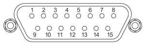
| Pin | Description | Pin | Description |
|---|---|---|---|
| 1 | Quadrature A- | 9 | Ground |
| 2 | Quadrature A+ | 10 | Motor Phase C (Black) |
| 3 | Quadrature B+ | 11 | Motor Phase A (Red) |
| 4 | Quadrature B- | 12 | Motor Phase B (White) |
| 5 | Encoder Index I- | 13 | +5 V |
| 6 | Encoder Index I+ | 14 | Ground |
| 7 | Negative Limit | 15 | Stage ID |
| 8 | Positive Limit | - | - |
Thorlabs offers two platforms to drive our wide range of motion controllers: our Kinesis® software package or the legacy APT™ (Advanced Positioning Technology) software package. Either package can be used to control devices in the Kinesis family, which covers a wide range of motion controllers ranging from small, low-powered, single-channel drivers (such as the K-Cubes™ and T-Cubes™) to high-power, multi-channel, modular 19" rack nanopositioning systems (the APT Rack System).
The Kinesis Software features .NET controls which can be used by 3rd party developers working in the latest C#, Visual Basic, LabVIEW™, or any .NET compatible languages to create custom applications. Low-level DLL libraries are included for applications not expected to use the .NET framework. A Central Sequence Manager supports integration and synchronization of all Thorlabs motion control hardware.
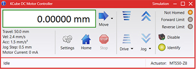
Kinesis GUI Screen
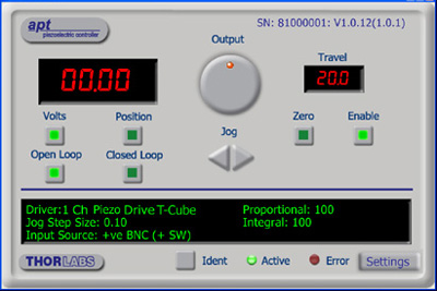
APT GUI Screen
Our legacy APT System Software platform offers ActiveX-based controls which can be used by 3rd party developers working on C#, Visual Basic, LabVIEW™, or any Active-X compatible languages to create custom applications and includes a simulator mode to assist in developing custom applications without requiring hardware.
By providing these common software platforms, Thorlabs has ensured that users can easily mix and match any of the Kinesis and APT controllers in a single application, while only having to learn a single set of software tools. In this way, it is perfectly feasible to combine any of the controllers from single-axis to multi-axis systems and control all from a single, PC-based unified software interface.
The software packages allow two methods of usage: graphical user interface (GUI) utilities for direct interaction with and control of the controllers 'out of the box', and a set of programming interfaces that allow custom-integrated positioning and alignment solutions to be easily programmed in the development language of choice.
A range of video tutorials is available to help explain our APT system software. These tutorials provide an overview of the software and the APT Config utility. Additionally, a tutorial video is available to explain how to select simulator mode within the software, which allows the user to experiment with the software without a controller connected. Please select the APT Tutorials tab above to view these videos.
Software
Kinesis Version 1.14.47
The Kinesis Software Package, which includes a GUI for control of Thorlabs' Kinesis and APT™ system controllers.
Also Available:
- Communications Protocol
Software
APT Version 3.21.6
The APT Software Package, which includes a GUI for control of Thorlabs' APT™ and Kinesis system controllers.
Also Available:
- Communications Protocol
Thorlabs' Kinesis® software features new .NET controls which can be used by third-party developers working in the latest C#, Visual Basic, LabVIEW™, or any .NET compatible languages to create custom applications.
C#
This programming language is designed to allow multiple programming paradigms, or languages, to be used, thus allowing for complex problems to be solved in an easy or efficient manner. It encompasses typing, imperative, declarative, functional, generic, object-oriented, and component-oriented programming. By providing functionality with this common software platform, Thorlabs has ensured that users can easily mix and match any of the Kinesis controllers in a single application, while only having to learn a single set of software tools. In this way, it is perfectly feasible to combine any of the controllers from the low-powered, single-axis to the high-powered, multi-axis systems and control all from a single, PC-based unified software interface.
The Kinesis System Software allows two methods of usage: graphical user interface (GUI) utilities for direct interaction and control of the controllers 'out of the box', and a set of programming interfaces that allow custom-integrated positioning and alignment solutions to be easily programmed in the development language of choice.
For a collection of example projects that can be compiled and run to demonstrate the different ways in which developers can build on the Kinesis motion control libraries, click on the links below. Please note that a separate integrated development environment (IDE) (e.g., Microsoft Visual Studio) will be required to execute the Quick Start examples. The C# example projects can be executed using the included .NET controls in the Kinesis software package (see the Kinesis Software tab for details).
 |
Click Here for the Kinesis with C# Quick Start Guide Click Here for C# Example Projects Click Here for Quick Start Device Control Examples |
|
LabVIEW
LabVIEW can be used to communicate with any Kinesis- or APT-based controller via .NET controls. In LabVIEW, you build a user interface, known as a front panel, with a set of tools and objects and then add code using graphical representations of functions to control the front panel objects. The LabVIEW tutorial, provided below, provides some information on using the .NET controls to create control GUIs for Kinesis- and APT-driven devices within LabVIEW. It includes an overview with basic information about using controllers in LabVIEW and explains the setup procedure that needs to be completed before using a LabVIEW GUI to operate a device.
 |
Click Here to View the LabVIEW Guide Click Here to View the Kinesis with LabVIEW Overview Page |
|
The APT video tutorials available here fall into two main groups - one group covers using the supplied APT utilities and the second group covers programming the APT System using a selection of different programming environments.
Disclaimer: The videos below were originally produced in Adobe Flash. Following the discontinuation of Flash after 2020, these tutorials were re-recorded for future use. The Flash Player controls still appear in the bottom of each video, but they are not functional.
Every APT controller is supplied with the utilities APTUser and APTConfig. APTUser provides a quick and easy way of interacting with the APT control hardware using intuitive graphical control panels. APTConfig is an 'off-line' utility that allows various system wide settings to be made such as pre-selecting mechanical stage types and associating them with specific motion controllers.
APT User Utility
The first video below gives an overview of using the APTUser Utility. The OptoDriver single channel controller products can be operated via their front panel controls in the absence of a control PC. The stored settings relating to the operation of these front panel controls can be changed using the APTUser utility. The second video illustrates this process.
APT Config Utility
There are various APT system-wide settings that can be made using the APT Config utility, including setting up a simulated hardware configuration and associating mechanical stages with specific motor drive channels. The first video presents a brief overview of the APT Config application. More details on creating a simulated hardware configuration and making stage associations are present in the next two videos.
APT Programming
The APT Software System is implemented as a collection of ActiveX Controls. ActiveX Controls are language-independant software modules that provide both a graphical user interface and a programming interface. There is an ActiveX Control type for each type of hardware unit, e.g. a Motor ActiveX Control covers operation with any type of APT motor controller (DC or stepper). Many Windows software development environments and languages directly support ActiveX Controls, and, once such a Control is embedded into a custom application, all of the functionality it contains is immediately available to the application for automated operation. The videos below illustrate the basics of using the APT ActiveX Controls with LabVIEW, Visual Basic, and Visual C++. Note that many other languages support ActiveX including LabWindows CVI, C++ Builder, VB.NET, C#.NET, Office VBA, Matlab, HPVEE etc. Although these environments are not covered specifically by the tutorial videos, many of the ideas shown will still be relevant to using these other languages.
Visual Basic
Part 1 illustrates how to get an APT ActiveX Control running within Visual Basic, and Part 2 goes on to show how to program a custom positioning sequence.
LabVIEW
Full Active support is provided by LabVIEW and the series of tutorial videos below illustrate the basic building blocks in creating a custom APT motion control sequence. We start by showing how to call up the Thorlabs-supplied online help during software development. Part 2 illustrates how to create an APT ActiveX Control. ActiveX Controls provide both Methods (i.e. Functions) and Properties (i.e. Value Settings). Parts 3 and 4 show how to create and wire up both the methods and properties exposed by an ActiveX Control. Finally, in Part 5, we pull everything together and show a completed LabVIEW example program that demonstrates a custom move sequence.
Part 1: Accessing Online Help
Part 2: Creating an ActiveX Control
Part 3: Create an ActiveX Method
Part 4: Create an ActiveX Property
Part 5: How to Start an ActiveX Control
The following tutorial videos illustrate alternative ways of creating Method and Property nodes:
Create an ActiveX Method (Alternative)
Create an ActiveX Property (Alternative)
Visual C++
Part 1 illustrates how to get an APT ActiveX Control running within Visual C++, and Part 2 goes on to show how to program a custom positioning sequence.
MATLAB
For assistance when using MATLAB and ActiveX controls with the Thorlabs APT positioners, click here.
To further assist programmers, a guide to programming the APT software in LabVIEW is also available here.
PID Basics
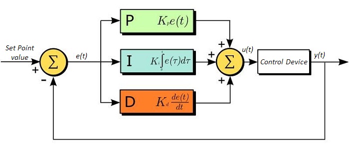
The PID circuit is often utilized as a control loop feedback controller and is very commonly used for many forms of servo circuits. The letters making up the acronym PID correspond to Proportional (P), Integral (I), and Derivative (D), which represents the three control settings of a PID circuit. The purpose of any servo circuit is to hold the system at a predetermined value (set point) for long periods of time. The PID circuit actively controls the system so as to hold it at the set point by generating an error signal that is essentially the difference between the set point and the current value. The three controls relate to the time-dependent error signal; at its simplest, this can be thought of as follows: Proportional is dependent upon the present error, Integral is dependent upon the accumulation of past error, and Derivative is the prediction of future error. The results of each of the controls are then fed into a weighted sum, which then adjusts the output of the circuit, u(t). This output is fed into a control device, its value is fed back into the circuit, and the process is allowed to actively stabilize the circuit’s output to reach and hold at the set point value. The block diagram below illustrates very simply the action of a PID circuit. One or more of the controls can be utilized in any servo circuit depending on system demand and requirement (i.e., P, I, PI, PD, or PID).
Through proper setting of the controls in a PID circuit, relatively quick response with minimal overshoot (passing the set point value) and ringing (oscillation about the set point value) can be achieved. Let’s take as an example a temperature servo, such as that for temperature stabilization of a laser diode. The PID circuit will ultimately servo the current to a Thermo Electric Cooler (TEC) (often times through control of the gate voltage on an FET). Under this example, the current is referred to as the Manipulated Variable (MV). A thermistor is used to monitor the temperature of the laser diode, and the voltage over the thermistor is used as the Process Variable (PV). The Set Point (SP) voltage is set to correspond to the desired temperature. The error signal, e(t), is then just the difference between the SP and PV. A PID controller will generate the error signal and then change the MV to reach the desired result. If, for instance, e(t) states that the laser diode is too hot, the circuit will allow more current to flow through the TEC (proportional control). Since proportional control is proportional to e(t), it may not cool the laser diode quickly enough. In that event, the circuit will further increase the amount of current through the TEC (integral control) by looking at the previous errors and adjusting the output in order to reach the desired value. As the SP is reached [e(t) approaches zero], the circuit will decrease the current through the TEC in anticipation of reaching the SP (derivative control).
Please note that a PID circuit will not guarantee optimal control. Improper setting of the PID controls can cause the circuit to oscillate significantly and lead to instability in control. It is up to the user to properly adjust the PID gains to ensure proper performance.
PID Theory
The output of the PID control circuit, u(t), is given as
where
Kp= Proportional Gain
Ki = Integral Gain
Kd = Derivative Gain
e(t) = SP - PV(t)
From here we can define the control units through their mathematical definition and discuss each in a little more detail. Proportional control is proportional to the error signal; as such, it is a direct response to the error signal generated by the circuit:
Larger proportional gain results is larger changes in response to the error, and thus affects the speed at which the controller can respond to changes in the system. While a high proportional gain can cause a circuit to respond swiftly, too high a value can cause oscillations about the SP value. Too low a value and the circuit cannot efficiently respond to changes in the system.
Integral control goes a step further than proportional gain, as it is proportional to not just the magnitude of the error signal but also the duration of the error.
Integral control is highly effective at increasing the response time of a circuit along with eliminating the steady-state error associated with purely proportional control. In essence integral control sums over the previous error, which was not corrected, and then multiplies that error by Ki to produce the integral response. Thus, for even small sustained error, a large aggregated integral response can be realized. However, due to the fast response of integral control, high gain values can cause significant overshoot of the SP value and lead to oscillation and instability. Too low and the circuit will be significantly slower in responding to changes in the system.
Derivative control attempts to reduce the overshoot and ringing potential from proportional and integral control. It determines how quickly the circuit is changing over time (by looking at the derivative of the error signal) and multiplies it by Kd to produce the derivative response.
Unlike proportional and integral control, derivative control will slow the response of the circuit. In doing so, it is able to partially compensate for the overshoot as well as damp out any oscillations caused by integral and proportional control. High gain values cause the circuit to respond very slowly and can leave one susceptible to noise and high frequency oscillation (as the circuit becomes too slow to respond quickly). Too low and the circuit is prone to overshooting the SP value. However, in some cases overshooting the SP value by any significant amount must be avoided and thus a higher derivative gain (along with lower proportional gain) can be used. The chart below explains the effects of increasing the gain of any one of the parameters independently.
| Parameter Increased | Rise Time | Overshoot | Settling Time | Steady-State Error | Stability |
|---|---|---|---|---|---|
| Kp | Decrease | Increase | Small Change | Decrease | Degrade |
| Ki | Decrease | Increase | Increase | Decrease Significantly | Degrade |
| Kd | Minor Decrease | Minor Decrease | Minor Decrease | No Effect | Improve (for small Kd) |
Tuning
In general the gains of P, I, and D will need to be adjusted by the user in order to best servo the system. While there is not a static set of rules for what the values should be for any specific system, following the general procedures should help in tuning a circuit to match one’s system and environment. In general a PID circuit will typically overshoot the SP value slightly and then quickly damp out to reach the SP value.
Manual tuning of the gain settings is the simplest method for setting the PID controls. However, this procedure is done actively (the PID controller turned on and properly attached to the system) and requires some amount of experience to fully integrate. To tune your PID controller manually, first the integral and derivative gains are set to zero. Increase the proportional gain until you observe oscillation in the output. Your proportional gain should then be set to roughly half this value. After the proportional gain is set, increase the integral gain until any offset is corrected for on a time scale appropriate for your system. If you increase this gain too much, you will observe significant overshoot of the SP value and instability in the circuit. Once the integral gain is set, the derivative gain can then be increased. Derivative gain will reduce overshoot and damp the system quickly to the SP value. If you increase the derivative gain too much, you will see large overshoot (due to the circuit being too slow to respond). By playing with the gain settings, you can maximize the performance of your PID circuit, resulting in a circuit that quickly responds to changes in the system and effectively damps out oscillation about the SP value.
| Control Type | Kp | Ki | Kd |
|---|---|---|---|
| P | 0.50 Ku | - | - |
| PI | 0.45 Ku | 1.2 Kp/Pu | - |
| PID | 0.60 Ku | 2 Kp/Pu | KpPu/8 |
While manual tuning can be very effective at setting a PID circuit for your specific system, it does require some amount of experience and understanding of PID circuits and response. The Ziegler-Nichols method for PID tuning offers a bit more structured guide to setting PID values. Again, you’ll want to set the integral and derivative gain to zero. Increase the proportional gain until the circuit starts to oscillate. We will call this gain level Ku. The oscillation will have a period of Pu. Gains are for various control circuits are then given below in the chart.
| Posted Comments: | |
涛 王
(posted 2023-12-25 18:17:38.867) I purchased two DDR25/M products from your company, both of which have problems. This has caused me a lot of distress. The first product has an issue with resetting, where the rotating table keeps rotating without stopping. I have already sent this product to your company for repair, but it has been a month and it is still not fixed. The second product has recently developed an issue where it displays “MGMSG HW RICHRESPONSE received: Phase initialization failed, motor cannot be enabled” when connected.
I really want to know what caused these problems and what measures I should take to prevent them from recurring. After all, every maintenance takes a long time, thank you! cstroud
(posted 2024-01-15 07:39:58.0) Thank you for reaching out, I'm sorry to hear about these issues. I will reach out to you directly to discuss troubleshooting options. Young Soo Yu
(posted 2023-11-29 14:53:22.533) Is this motorized mount usable in vacuum conditions? do'neill
(posted 2023-12-01 09:53:43.0) Response from Daniel at Thorlabs. The DDR25(/M) is not vacuum compatible, the closest stage that would be compatible is probably the PDR1V(/M). I will reach out to you directly to discuss your application. user
(posted 2022-08-13 16:29:11.46) The overview says "The mount is designed to be mounted vertically on a post using one of four 8-32 (M4) taps on the sides of the device."
Does that mean it will not work if mounted horizontally, or will there be malfunctions? cwright
(posted 2022-08-15 10:06:30.0) Response from Charles at Thorlabs: Thank you for your query. There are 4x 4-40 holes on the back of the device which are intended for our cage rods. These can be used to mount the device vertically but weight should not hang from the front of the device. user
(posted 2022-03-26 17:11:49.38) It can't find the homing position and keeps turning. I can't use kinesis to control it Simon Neves
(posted 2022-02-18 11:29:08.173) We've had a DDR25/M for around 3 years, and everything was working fine until few days ago. Now it can't find the homing position and keeps turning. Do you know how to fix this problem? Thank you cwright
(posted 2022-02-22 03:29:07.0) Response from Charles at Thorlabs: Thank you for your query. Often this is caused by a moment load pulling on the front plate. This pulls the readhead away from the encoder and prevents homing. A member of technical support will contact you. CJ Lim
(posted 2020-10-16 14:47:58.943) Hi, may I check the dynamic torque range for this DDR25?
Thanks!
CJ cwright
(posted 2020-10-21 04:33:57.0) Response from Charles at Thorlabs:Hello and thank you for your query. Unfortunately this is not a specification we can currently provide. We will reach out to you directly to see if we can still assist with your application. Ryan Merrithew
(posted 2020-08-19 12:33:47.933) Do you have an estimate for the Mean Time Between Failures on the mount?
I'm interested in an application where my optic will be left spinning for long periods of time. DJayasuriya
(posted 2020-08-27 09:58:25.0) Thank you for your inquiry. The mean time failure would depend on couple of different factors. Usually the main factor being the bearings of the unit. We will get in touch with you directly to help with your application. FONG WAI LOON
(posted 2020-07-12 21:54:57.6) Do you have a value for the minimum incremental motion? cwright
(posted 2020-07-17 10:58:49.0) Response from Charles at Thorlabs: Thank you for your query. Unfortunately we do not specify a value for minimum incremental motion at this time. Jeff Chen
(posted 2020-06-18 20:52:52.533) Hi,
The stage sometimes took about 15 minutes to find the home position. How to solve this issue? DJayasuriya
(posted 2020-06-22 04:36:45.0) Thank you for your inquiry. We will get in touch with you directly to get this resolved. Scott Snider
(posted 2020-01-08 18:10:49.38) This STEP file has errors in it. Doesn't import properly to NX12 AManickavasagam
(posted 2020-01-29 03:49:24.0) Response from Arunthathi at Thorlabs: Thanks for your query. We have double checked the STEP file and looks like there are no errors and would most likely be to do with compatibility issues when trying to import to NX12. Looks like STEP files can be opened directly in NX12 just using the File→Open command and changing the “Files of type” filter: Select File→Import→STEP203, STEP214, or STEP242. I have also contacted you directly with the file types that could work. Emmanuel Mazy
(posted 2019-10-23 05:25:19.853) What is the accuracy of the homing of the rotation stage ? cwright
(posted 2019-10-23 09:17:17.0) Hello Emmanuel, thank you for contacting us. Unfortunately at this time we are not in a position to supply this specification but we are looking into providing it in due course. I will contact you directly to discuss your needs in more detail. moran5
(posted 2019-02-21 20:27:03.613) I see the velocity stability is spec'ed at ± 2° for speeds between 0.5-5Hz. How about slower speeds? For example can this stage run at slower speeds, like 10°/sec (0.0277Hz)? If so what might be its stability? I assume it is good at you mention a PID control loop and an encoder. What say you? rmiron
(posted 2019-02-28 05:51:19.0) Response from Radu at Thorlabs: Hello, Moran. From Kinesis, the minimum angular velocity that can be commanded is 0.01°/sec (~28μHz). Upon receiving such a command, the stage will rotate at an average of 0.01°/sec, but its velocity stability will be poor. Using low-level serial commands, you can order the stage to move at ~0.134 arcsecs/s (~103.5nHz). However, it is unlikely that the stage would move at all upon receiving such a command. We specify a 0.5-5Hz range because that is the range for which we can guarantee that the instantaneous velocity will consistently be within +/-2% of the demanded value. At 10°/sec we can no longer guarantee that, but we expect the instantaneous velocity to still be within +/-2% most of the time. Generally speaking, the lower the velocity, the poorer its stability. On a different note, you could try to improve velocity stability at lower speeds by decreasing the proportional gain or by increasing the derivative gain (at the expense of taking a longer time to reach target velocity). simon.neves
(posted 2018-10-18 11:21:39.893) Can we integrate a mounted 0.5" zero-order HWP in this system ? I see that the real size of such a wave plate is 1", because of the mount. Could we think of an unmounted version that could be integrated in this motor ?
Thank you very much rmiron
(posted 2018-10-19 10:49:53.0) Response from Radu at Thorlabs: Hello Simon. If your HWP has a total diameter of 1", then you cannot mount it directly. However, given our range of products, it is certainly possible to mount it with the aid of some adapters. I will contact you via email in order discuss what adapters would be necessary in your case. a.brash
(posted 2018-10-04 16:11:21.837) Do you have a value for the minimum incremental motion? rmiron
(posted 2018-10-05 05:18:47.0) Response from Radu at Thorlabs: Unfortunately, we don't have this specification at the moment. We are aware that it is an important parameter when deciding whether to purchase a rotation stage. Consequently, we are working on addressing this lack of information and the specification should be on the website shortly. I will contact you directly in order to provide more details. thomas.mattes
(posted 2016-11-21 10:07:24.52) is a product like this with similar high rotation speed is available for bigger optical Diameters about 30 mm?
Best Regards
Thomas Mattes bwood
(posted 2016-11-22 06:59:16.0) Response from Ben at Thorlabs: Thank you for your question. The DRR100 is a comparable rotation mount, which offers similar speeds (3Hz) with a SM1 threaded central aperture. This is the largest optic diameter, high speed mount we can offer, and it can be found on our website here: https://www.thorlabs.de/newgrouppage9.cfm?objectgroup_id=8184 user
(posted 2016-06-27 04:14:53.113) In addition to the wobble, do you have the eccentricity error in micrometer? Thanks. tfrisch
(posted 2016-07-01 03:23:18.0) Hello,
The radial run out is 12um. |
Rotation Mount and Stage Selection Guide
Thorlabs offers a wide variety of manual and motorized rotation mounts and stages. Rotation mounts are designed with an inner bore to mount a Ø1/2", Ø1", or Ø2" optic, while rotation stages are designed with mounting taps to attach a variety of components or systems. Motorized options are powered by a DC Servo motor, 2 phase stepper motor, piezo inertia motor, or an Elliptec™ resonant piezo motor. Each offers 360° of continuous rotation.
Manual Rotation Mounts
| Rotation Mounts for Ø1/2" Optics | |||||||
|---|---|---|---|---|---|---|---|
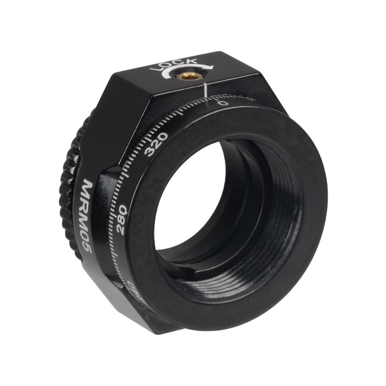
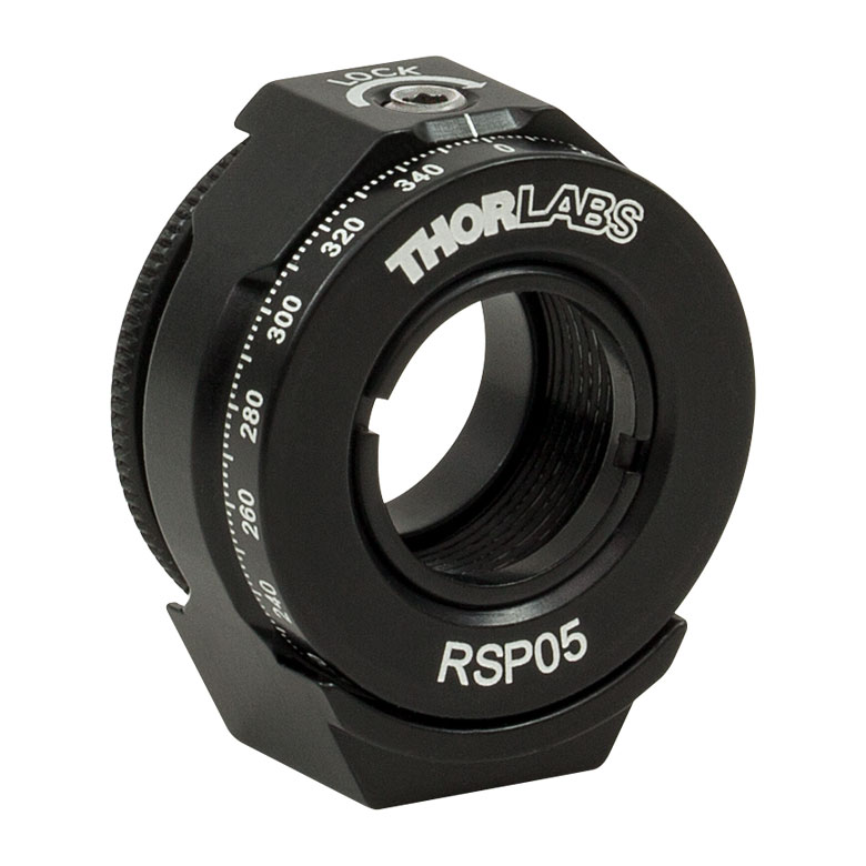
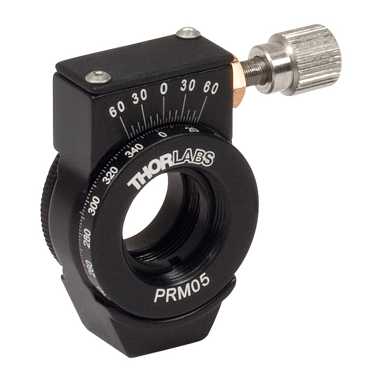
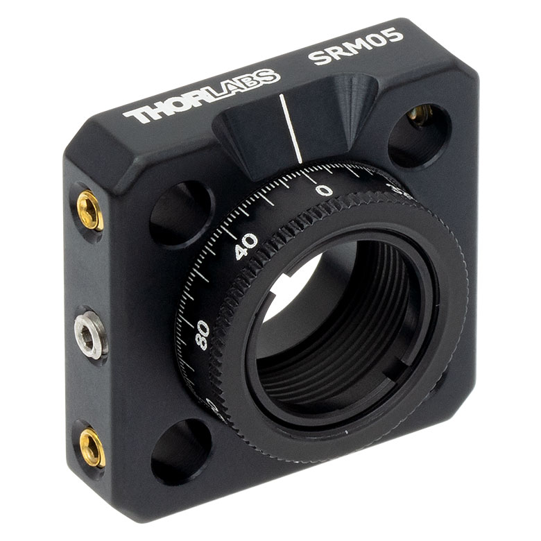
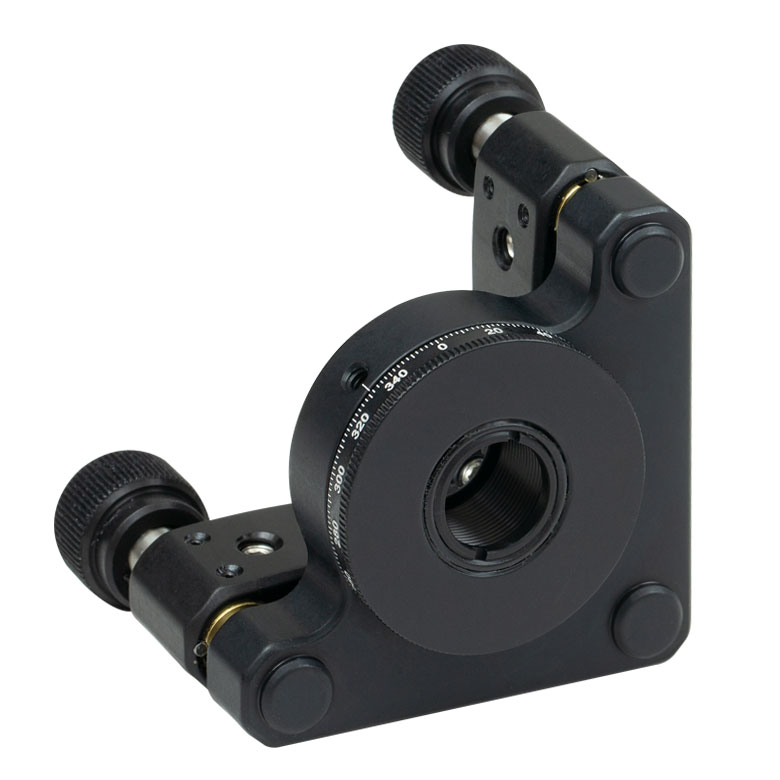
| Item # | MRM05(/M) | RSP05(/M) | CRM05 | PRM05(/M)a | SRM05 | KS05RS | CT104 |
| Click Photo to Enlarge |
 |
 |
 |
 |
 |
 |
 |
| Features | Mini Series | Standard | External SM1 (1.035"-40) Threads |
Micrometer | 16 mm Cage-Compatible | ±4° Kinematic Tip/Tilt Adjustment Plus Rotation | Compatible with 30 mm Cage Translation Stages and 1/4" Translation Stagesb |
| Additional Details | |||||||
| Rotation Mounts for Ø1" Optics | ||||||||
|---|---|---|---|---|---|---|---|---|
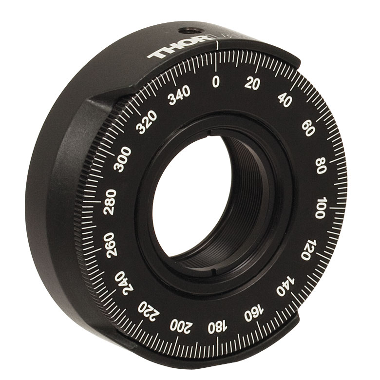
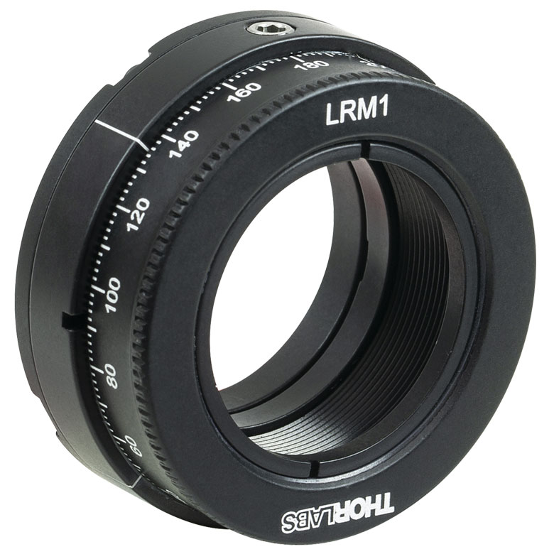
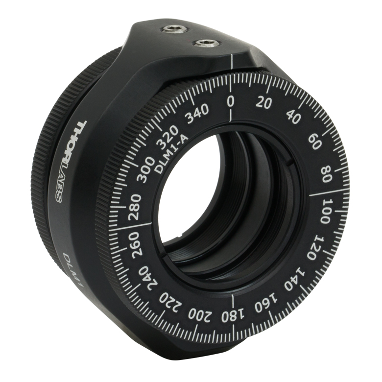
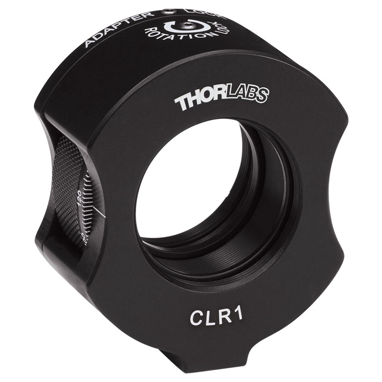
| Item # | RSP1(/M) | LRM1 | RSP1D(/M) | DLM1(/M) | CLR1(/M) | RSP1X15(/M) | RSP1X225(/M) | PRM1(/M)a |
| Click Photo to Enlarge |
 |
 |
 |
 |
 |
 |
|
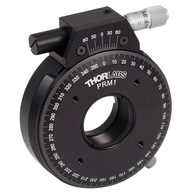 |
| Features | Standard | External SM1 (1.035"-40) Threads |
Adjustable Zero | Two Independently Rotating Carriages | Rotates Optic Within Fixed Lens Tube System |
Continuous 360° Rotation or 15° Increments |
Continuous 360° Rotation or 22.5° Increments |
Micrometer |
| Additional Details | ||||||||
| Rotation Mounts for Ø1" Optics | ||||||
|---|---|---|---|---|---|---|
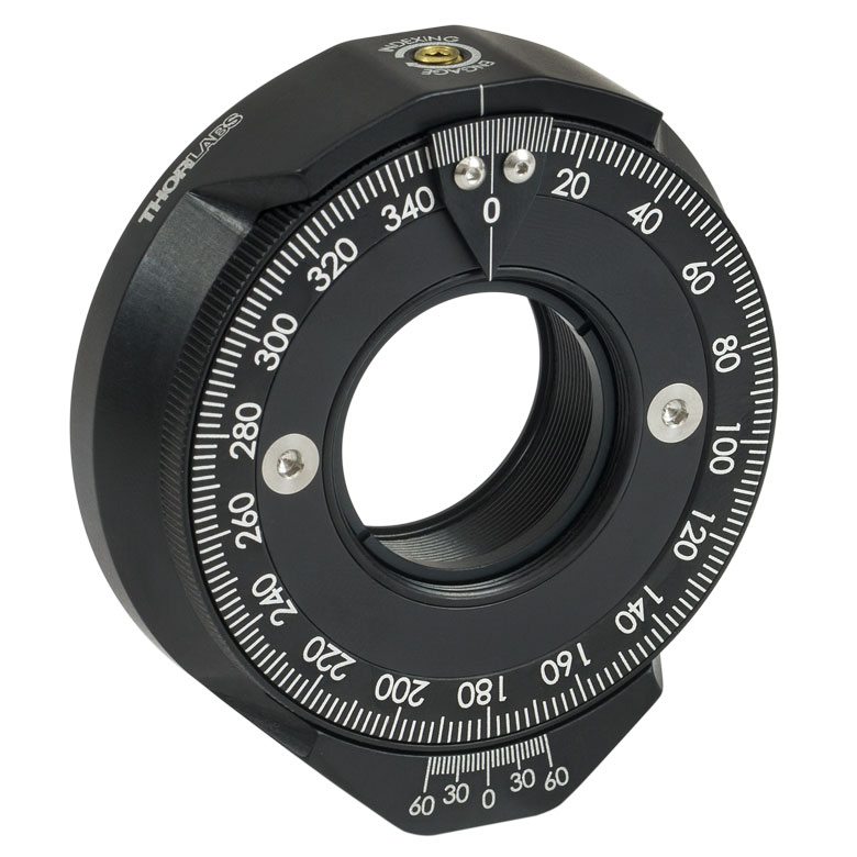
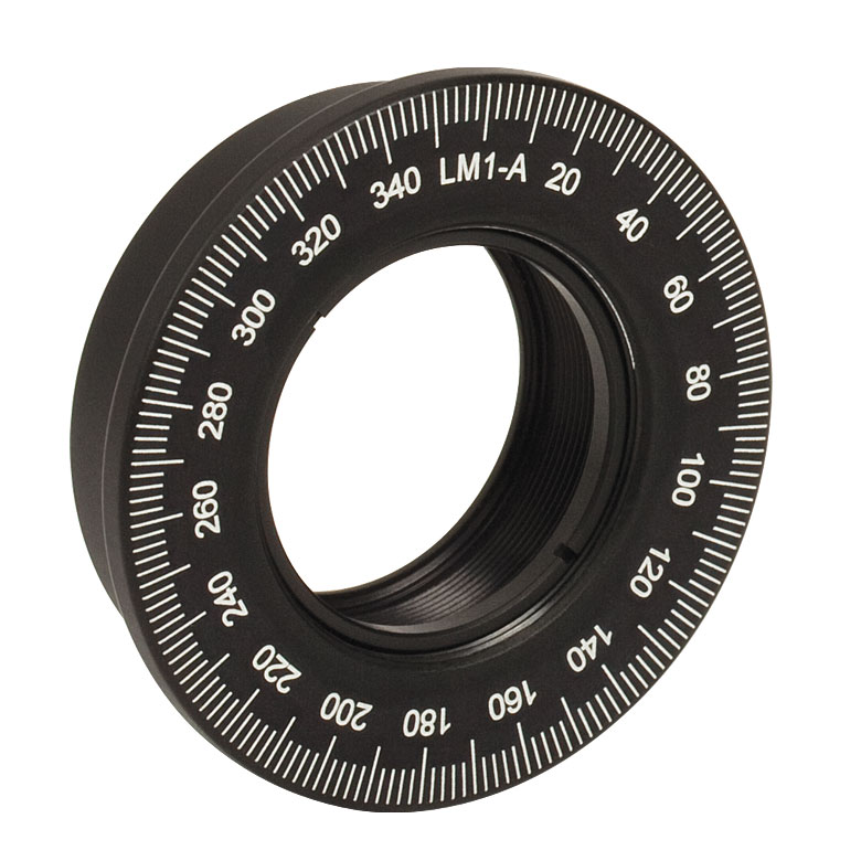
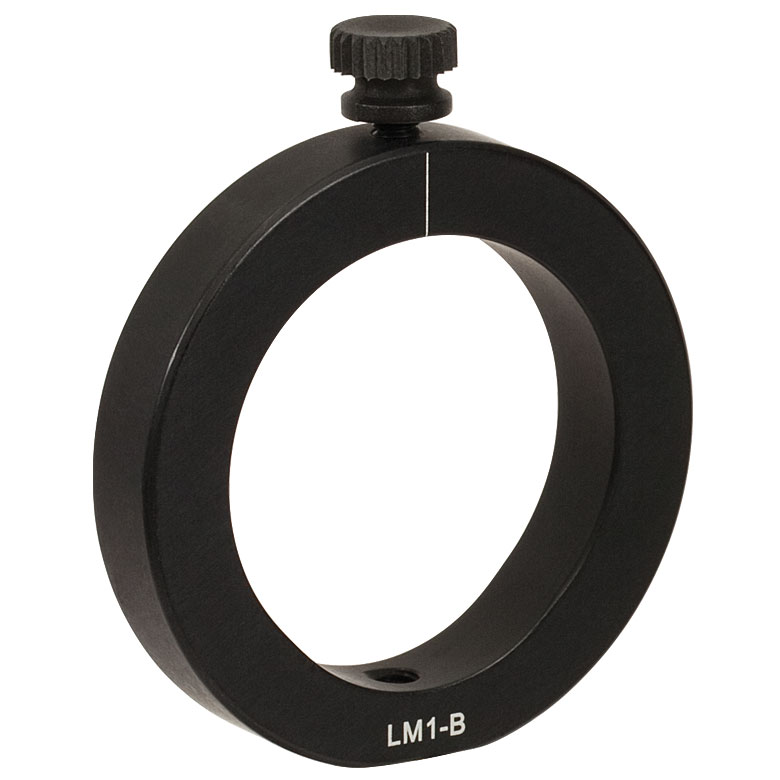
| Item # | LM1-A & LM1-B(/M) |
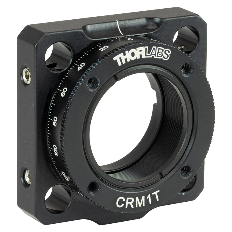
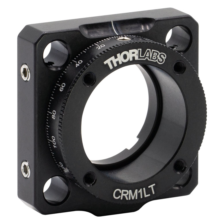
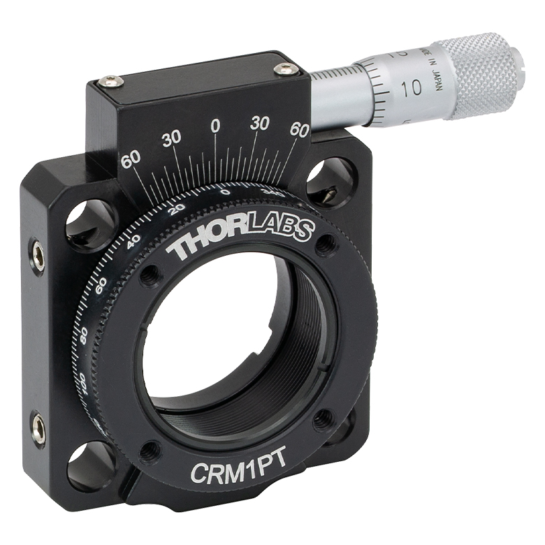
CRM1T(/M) | CRM1LT(/M) | CRM1PT(/M) | KS1RS | K6XS |
| Click Photo to Enlarge |
  |
 |
 |
 |
 |
 |
| Features | Optic Carriage Rotates Within Mounting Ring | 30 mm Cage-Compatiblea | 30 mm Cage-Compatible for Thick Opticsa |
30 mm Cage-Compatible with Micrometera |
±4° Kinematic Tip/Tilt Adjustment Plus Rotation | Six-Axis Kinematic Mounta |
| Additional Details | ||||||
| Rotation Mounts for Ø2" Optics | |||||||
|---|---|---|---|---|---|---|---|
| Item # | RSP2(/M) | RSP2D(/M) | PRM2(/M) | LM2-A & LM2-B(/M) |
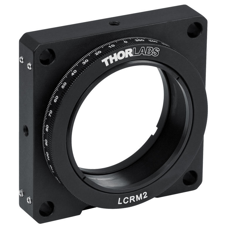
LCRM2(/M) | KS2RS | K6X2 |
| Click Photo to Enlarge |  |
 |
 |
  |
 |
 |
 |
| Features | Standard | Adjustable Zero |
Micrometer | Optic Carriage Rotates Within Mounting Ring | 60 mm Cage-Compatible | ±4° Kinematic Tip/Tilt Adjustment Plus Rotation | Six-Axis Kinematic Mount |
| Additional Details | |||||||
Manual Rotation Stages
| Manual Rotation Stages | ||||||
|---|---|---|---|---|---|---|
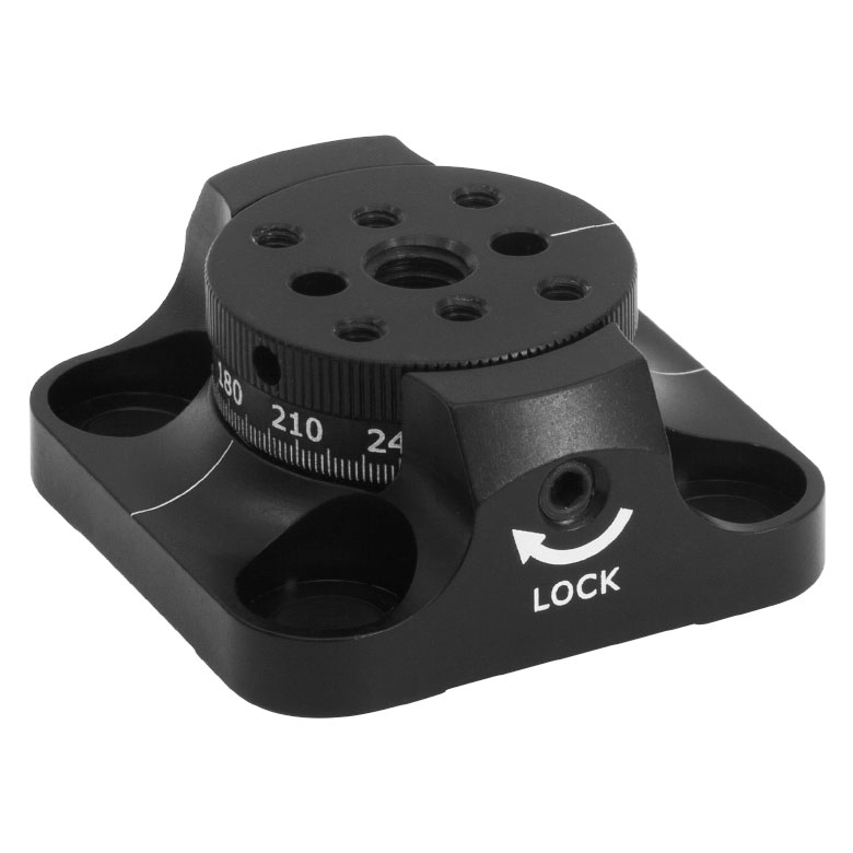
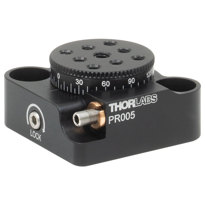
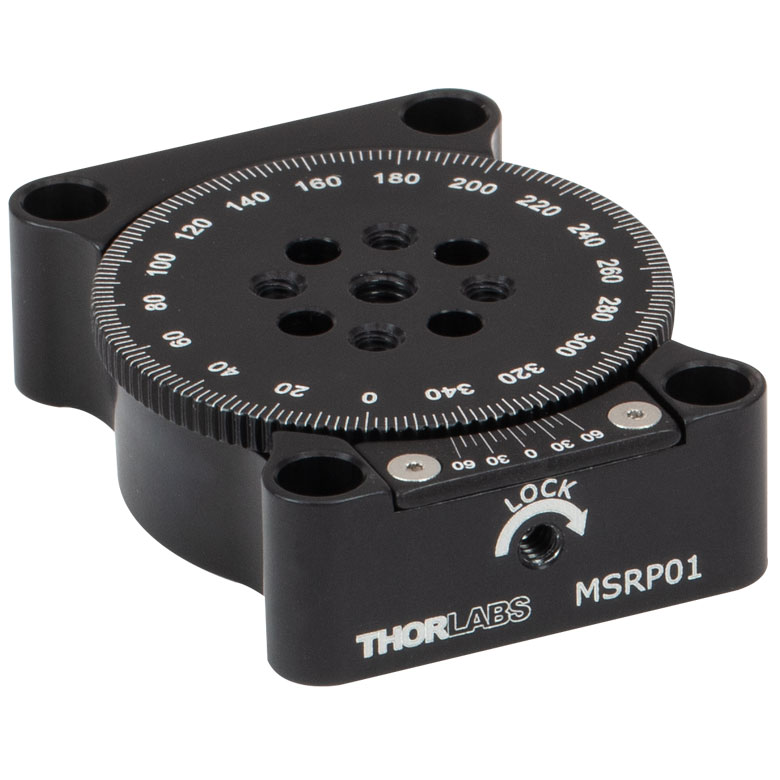
| Item # | RP005(/M) | PR005(/M) | MSRP01(/M) | RP01(/M) | RP03(/M) | QRP02(/M) |
| Click Photo to Enlarge |
 |
 |
 |
 |
 |
 |
| Features | Standard | Two Hard Stops | ||||
| Additional Details | ||||||
| Manual Rotation Stages | ||||||
|---|---|---|---|---|---|---|
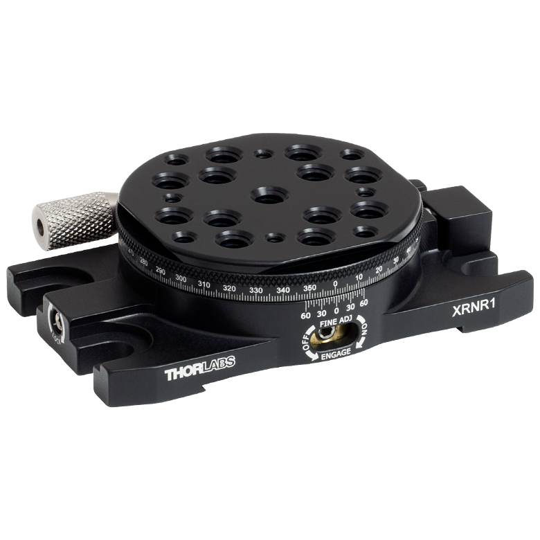
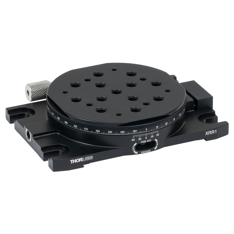
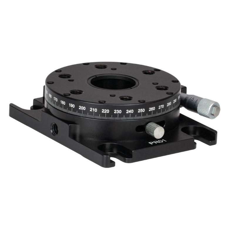
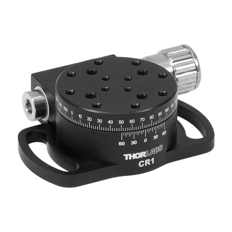
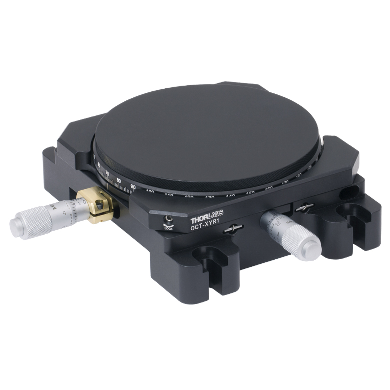
| Item # | XRNR1(/M) | XRR1(/M) | PR01(/M) | CR1(/M) | XYR1(/M) | OCT-XYR1(/M) |
| Click Photo to Enlarge |
 |
 |
 |
 |
 |
 |
| Features | Fine Rotation Adjuster and 2" Wide Dovetail Quick Connect |
Fine Rotation Adjuster and 3" Wide Dovetail Quick Connect |
Fine Rotation Adjuster and SM1-Threaded Central Aperture |
Fine Pitch Worm Gear | Rotation and 1/2" Linear XY Translation | |
| Additional Details | ||||||
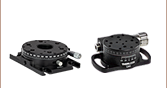
Motorized Rotation Mounts and Stages
| Motorized Rotation Mounts and Stages with Central Clear Apertures | |||||
|---|---|---|---|---|---|
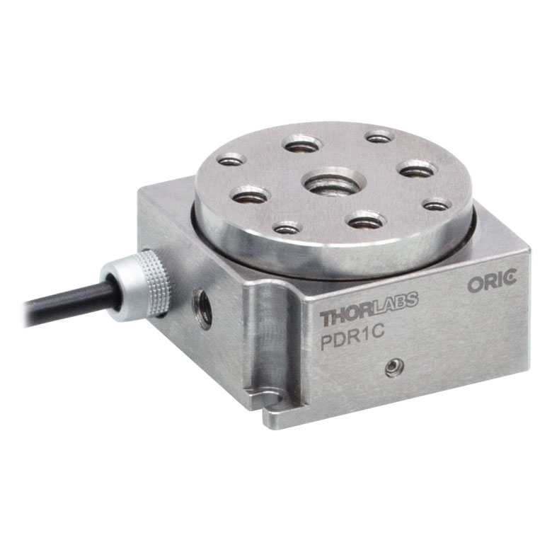
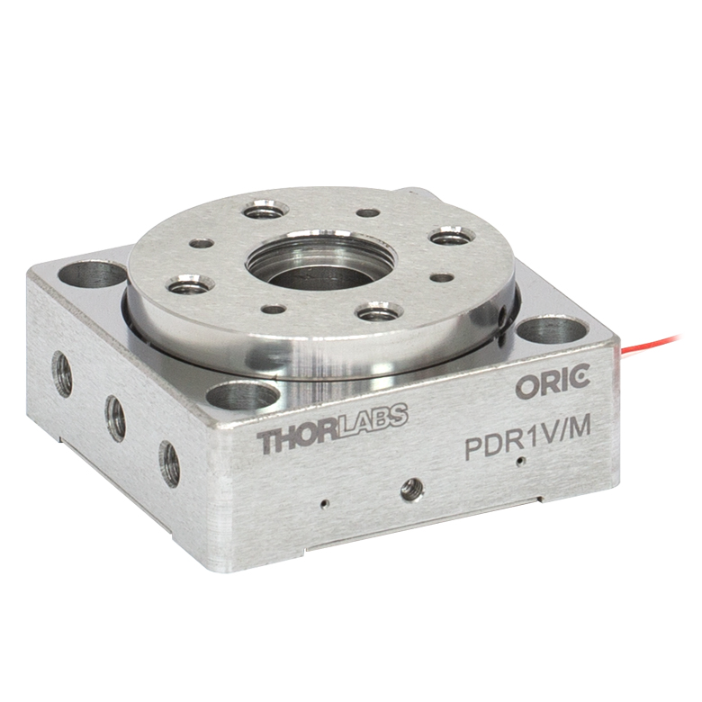
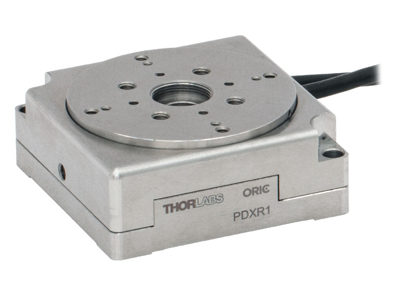
| Item # | DDR25(/M) | PDR1C(/M) | PDR1(/M) | PDR1V(/M) | PDXR1(/M) |
| Click Photo to Enlarge |
 |
 |
 |
 |
 |
| Features | Compatible with SM05 Lens Tubes, 16 mm Cage System, & 30 mm Cage System |
Compatible with 16 mm Cage System |
Compatible with SM05 Lens Tubes & 30 mm Cage System |
Vacuum-Compatible; Also Compatible with SM05 Lens Tubes & 30 mm Cage System |
Compatible with SM05 Lens Tubes & 30 mm Cage System |
| Additional Details | |||||
| Motorized Rotation Mounts and Stages with Central Clear Apertures | |||||
|---|---|---|---|---|---|
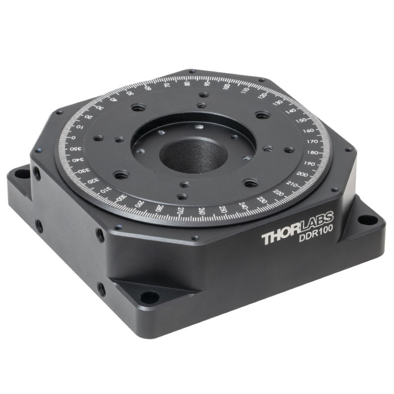
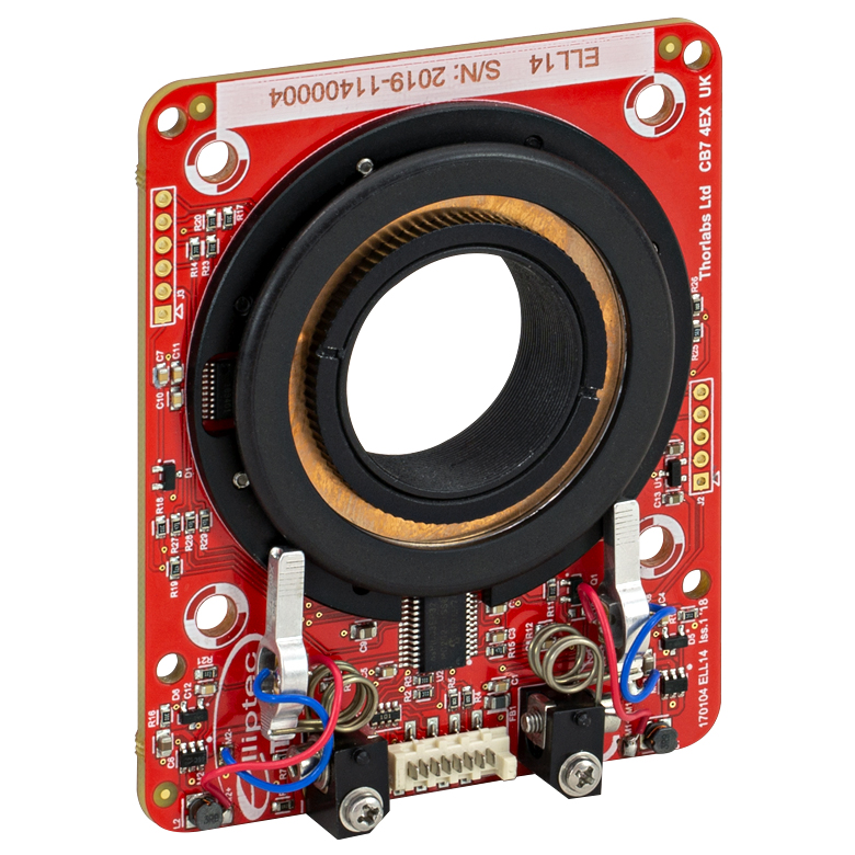
| Item # | K10CR1(/M) | PRM1Z8(/M)a | DDR100(/M) | ELL14 | HDR50(/M) |
| Click Photo to Enlarge |
 |
 |
 |
 |
 |
| Features | Compatible with SM1 Lens Tubes & 30 mm Cage System | Compatible with SM1 Lens Tubes, 16 mm Cage System, 30 mm Cage System |
Compatible with SM1 Lens Tubes, Open Frame Design for OEM Applications |
Compatible with SM2 Lens Tubes |
|
| Additional Details | |||||
| Motorized Rotation Mounts and Stages with Tapped Platforms | ||
|---|---|---|
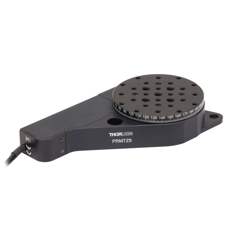
| Item # | PRMTZ8(/M)a | ELL18(/M)b |
| Click Photo to Enlarge |
 |
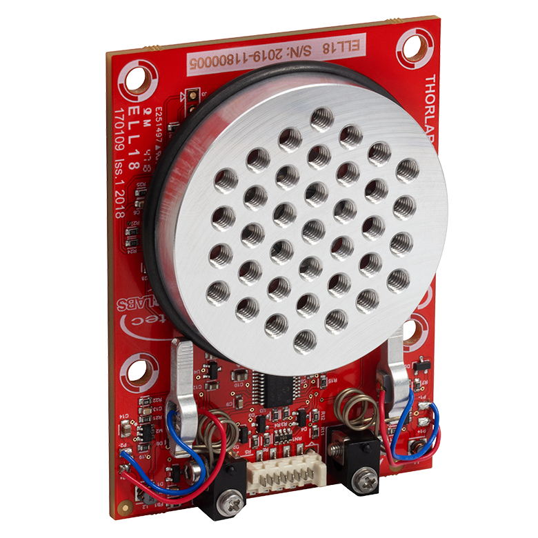 |
| Features | Tapped Mounting Platform for Mounting Prisms or Other Optics | Tapped Mounting Platform, Open Frame Design for OEM Applications |
| Additional Details | ||

 Zoom
Zoom
Click to Enlarge
Diagram Showing the Dimensions of the DDR25(/M) Rotation Stage and the Position of Tapped Holes for Cage System Rods
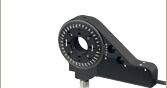
- Rotational Speeds up to 5.0 Hz (1800 °/s)
- Integrated Brushless DC Servo Motor
- SM05 (0.535"-40) Threaded Bore for Ø1/2" Lens Tubes
- 16 mm and 30 mm Cage System Compatible
- Four 8-32 (M4) Mounting Holes
- Driver Not Included (See Below)
Characterized by high-speed rotation and high-positional accuracy, the DDR25(/M) mount is well-suited for applications where there is a need to rotate components at high speed within a cage or other system. This mount is driven by the KBD101 brushless DC controller (sold separately below), which provides precise positioning through the stable closed-loop PID control system.

 Zoom
Zoom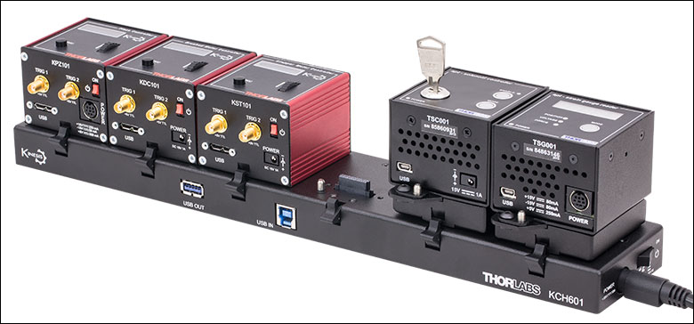
Click to Enlarge
KCH601 USB Controller Hub (Sold Separately) with Installed K-Cube and T-Cube™ Modules (T-Cubes shown on the KAP101 Adapter)
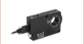
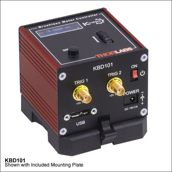
- Front Panel Velocity Wheel and Digital Display for Controlling Motorized Stages or Actuators
- Two Bidirectional SMC Trigger Ports to Read or Control External Equipment
- Interfaces with Computer Using Included USB Cable
- Fully Compatible with Kinesis® or APT™ Software Packages
- Compact Footprint: 60.0 mm x 60.0 mm x 49.2 mm (2.42" x 2.42" x 1.94")
- Power Supply Not Included (See Below)
Thorlabs' KBD101 K-Cube™ Brushless DC Motor Controller provides local and computerized control of a single motor axis. It features a top-mounted control panel with a velocity wheel that supports four-speed bidirectional control with forward and reverse jogging as well as position presets. A backlit digital display is also included that can have the backlit dimmed or turned off using the the top-panel menu options. The front of the unit contains two bidirectional SMC trigger ports that can be used to read a 5 V external logic signal or output a 5 V logic signal to control external equipment. Each port can be independently configured.
The unit is fully compatible with our new Kinesis software package and our legacy APT control software.
Please note that this controller does not ship with a power supply. Compatible power supplies are listed below. Additional information can be found on the main KBD101 Brushless DC Servo Motor Controller page.

 Zoom
Zoom
Click for Details
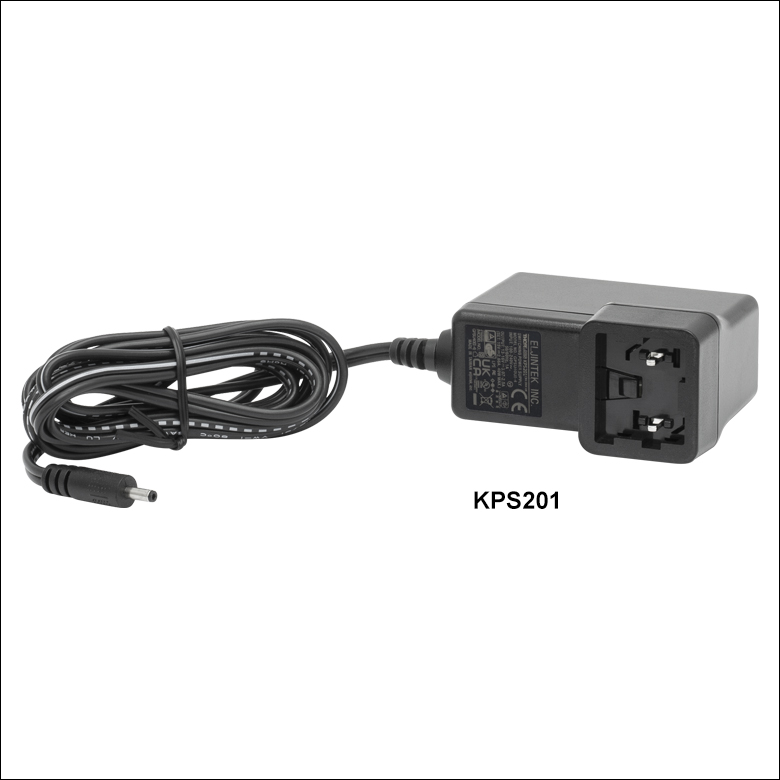
Each KPS201 power supply includes one region-specific adapter, which can be selected upon checkout.
Click to Enlarge
The KPS201 Power Supply Unit
- Individual Power Supply
- KPS201: For K-Cubes™ or T-Cubes™ with 3.5 mm Jacks
- USB Controller Hubs Provide Power and Communications
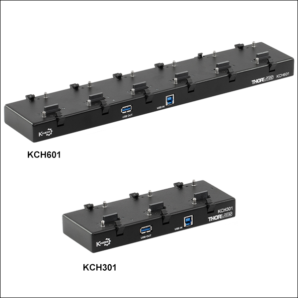
- KCH301: For up to Three K-Cubes or T-Cubes
- KCH601: For up to Six K-Cubes or T-Cubes
The KPS201 power supply outputs +15 VDC at up to 2.66 A and can power a single K-Cube or T-Cube with a 3.5 mm jack. It plugs into a standard wall outlet.
The KCH301 and KCH601 USB Controller Hubs each consist of two parts: the hub, which can support up to three (KCH301) or six (KCH601) K-Cubes or T-Cubes, and a power supply that plugs into a standard wall outlet. The hub draws a maximum current of 10 A; please verify that the cubes being used do not require a total current of more than 10 A. In addition, the hub provides USB connectivity to any docked K-Cube or T-Cube through a single USB connection.
For more information on the USB Controller Hubs, see the full web presentation.